Excel Power Query
What is Power Query?
Power Query is a tool that helps you collect data from different places, clean it up, and organize it the way you need. You can do this using a simple editor without writing code, and then load the data into Excel, Power BI, or other tools.
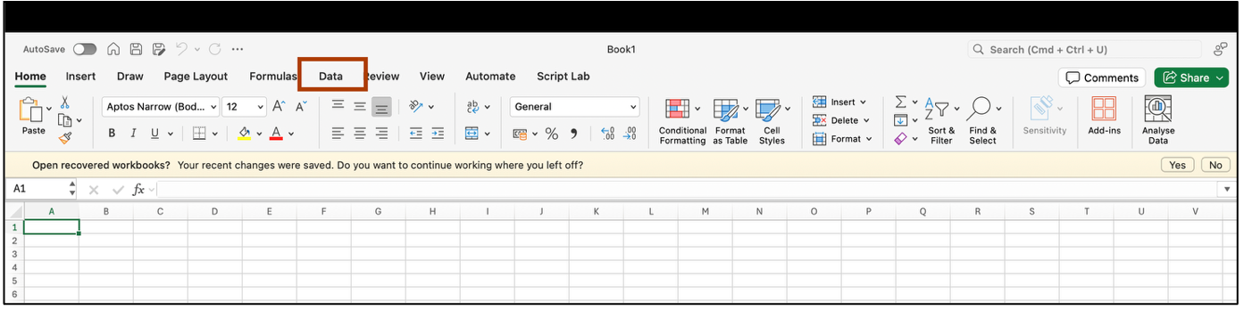
Where to find it in Excel?
• Open Excel
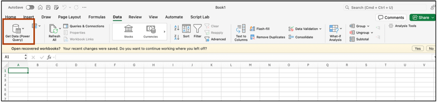
• Click on the Data at the Top Ribbon
• Click on Get Data (Power Query) to load data from different sources
Common Supported Data Sources in Power Query
• Excel Workbooks
• CSV files
• SQL Server
• SharePoint
• Azure and AWS data storage
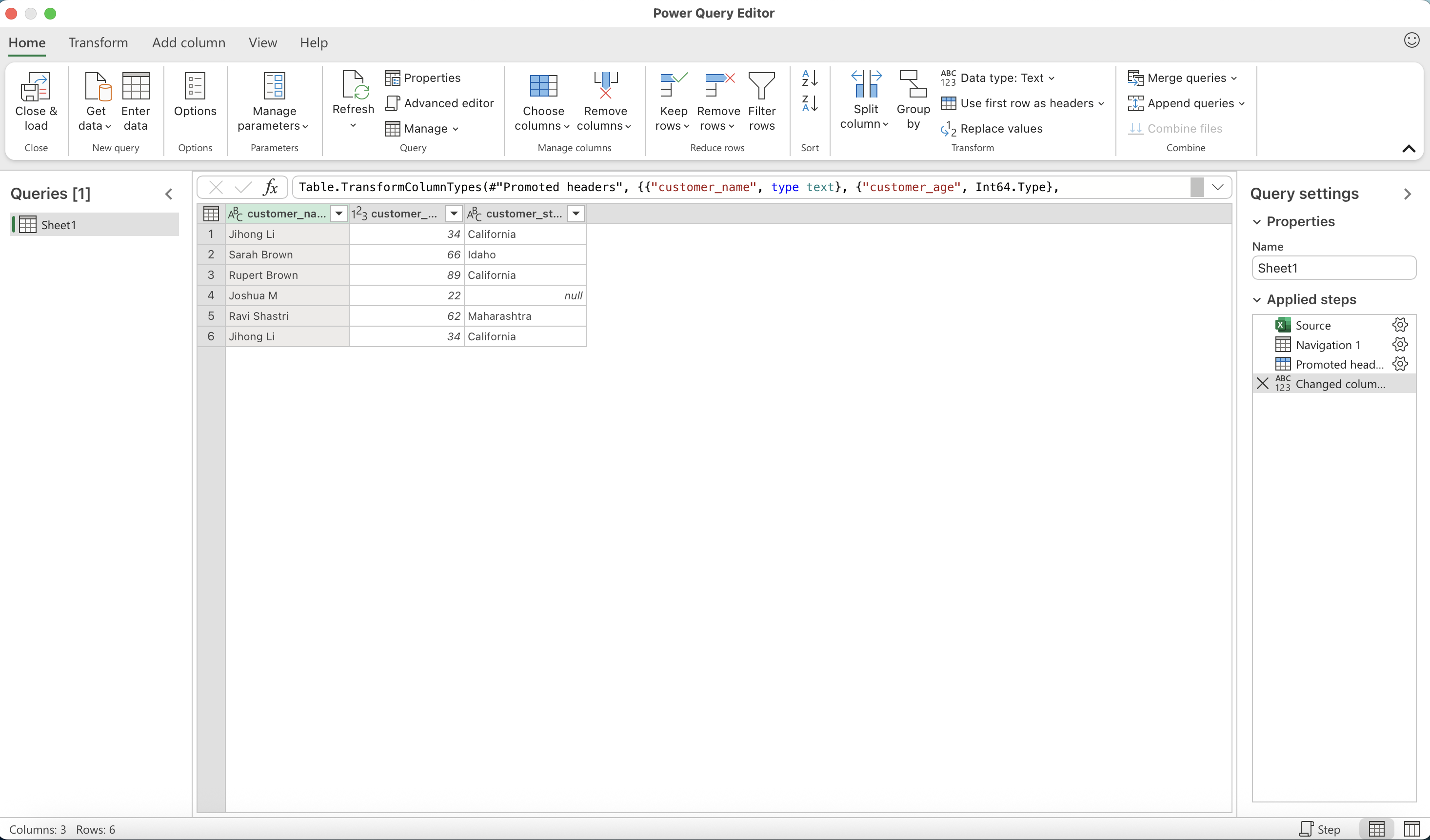
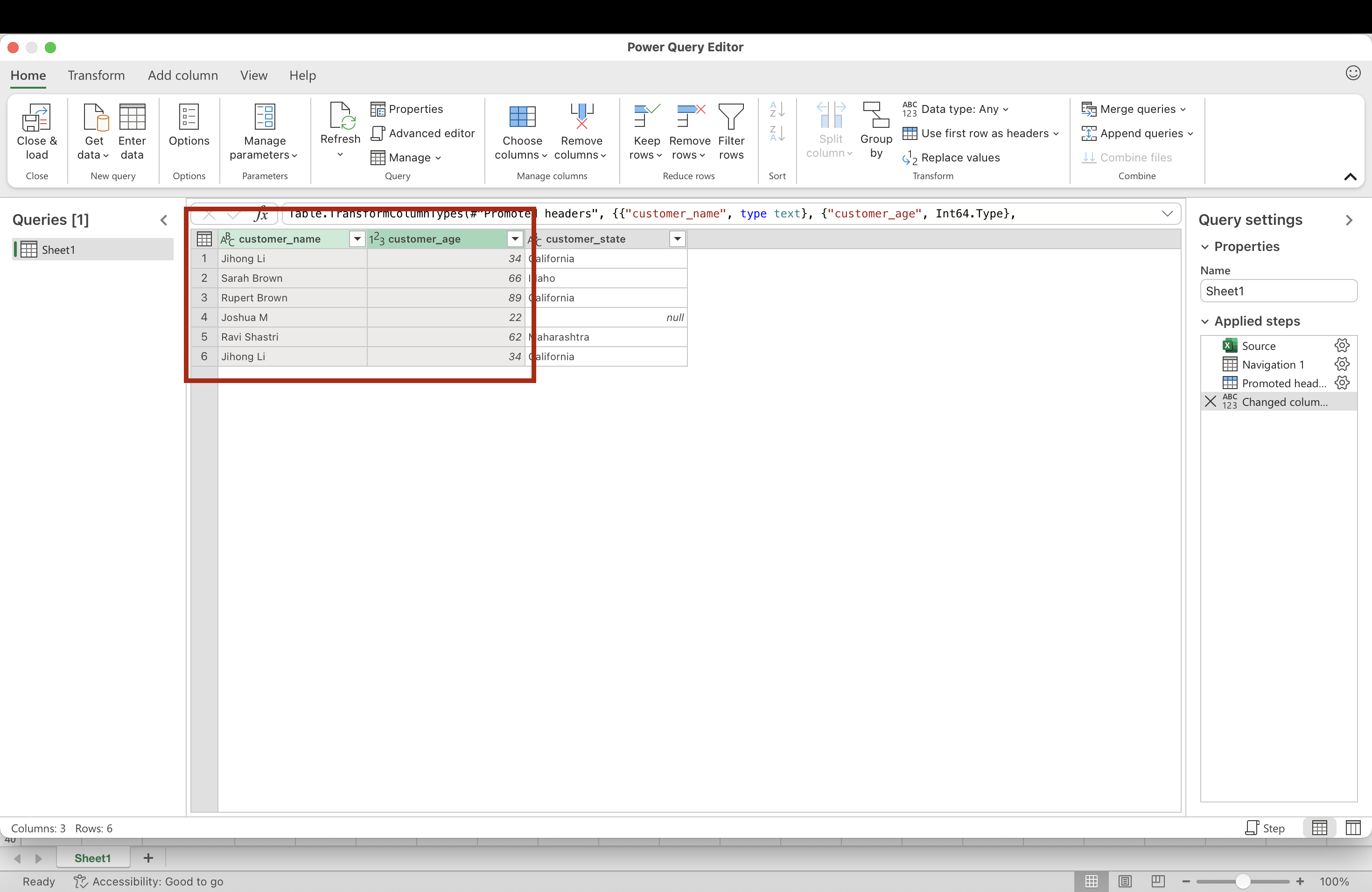
This is what the Power Query window looks like after loading your data:
Types of Transformations in Power Query:
1. Row Transformation: Changes applied to existing data rows. Example: filtering rows, removing duplicates, sorting, replacing values.
2. Column Transformations: Creates or modifies columns in your table. Example: adding a calculated column, splitting columns, extracting values from a column.
We will be working with this table to perform data transformation using Power query.
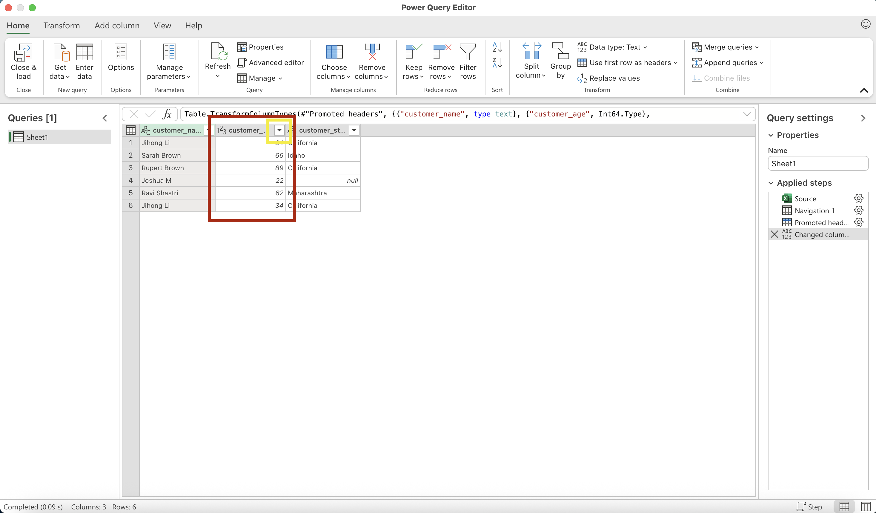
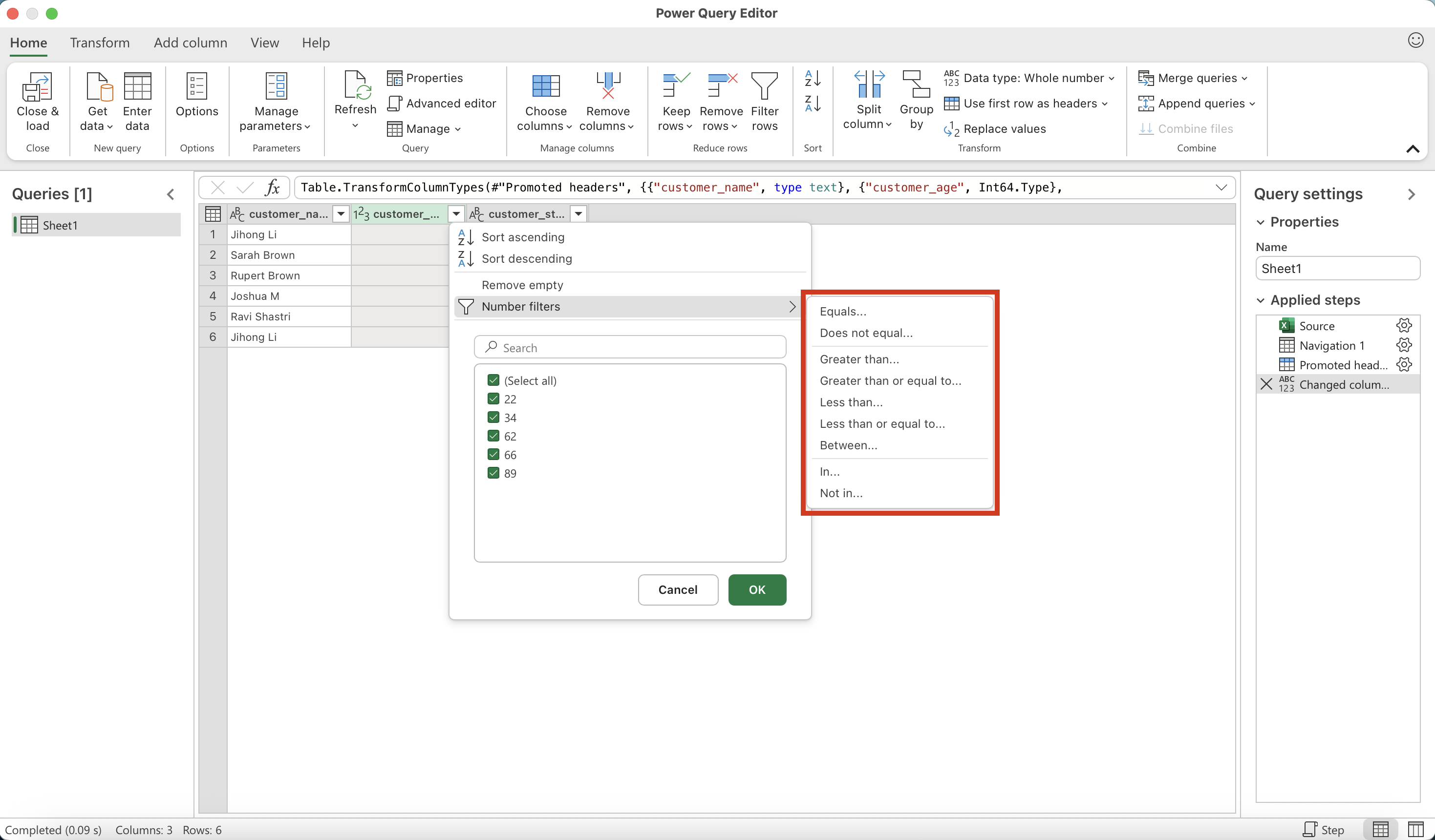
Excluding Rows: Filter
• Select the column you want to filter on
• Go to the column header and click the drop-down filter icon
• Choose the values or set conditions (e.g., “Equals”, “Greater Than”, etc.)
• Power Query will keep only the rows that meet your filter criteria
The Query Settings panel (on the right side) shows the name of your query and keeps track of every step you take while cleaning your data. It’s like a timeline of your work, easy to follow, easy to fix, and super helpful when you want to reuse or update your process later.
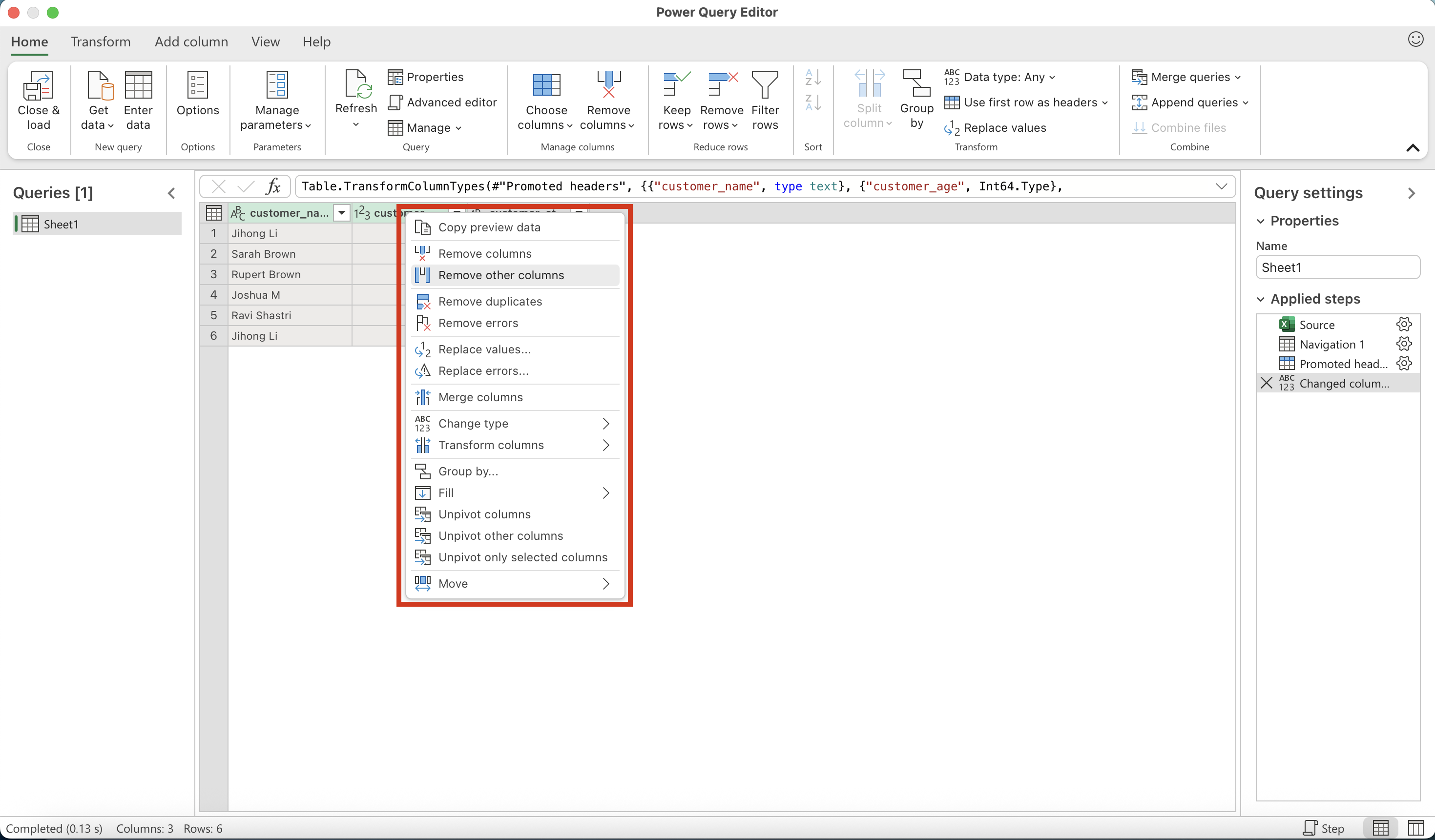
Excluding Columns: Select
• Go to the Home tab
• Select the columns you want to keep
• Right-click on a column header and choose Remove other columns
• Power Query will display only the selected columns
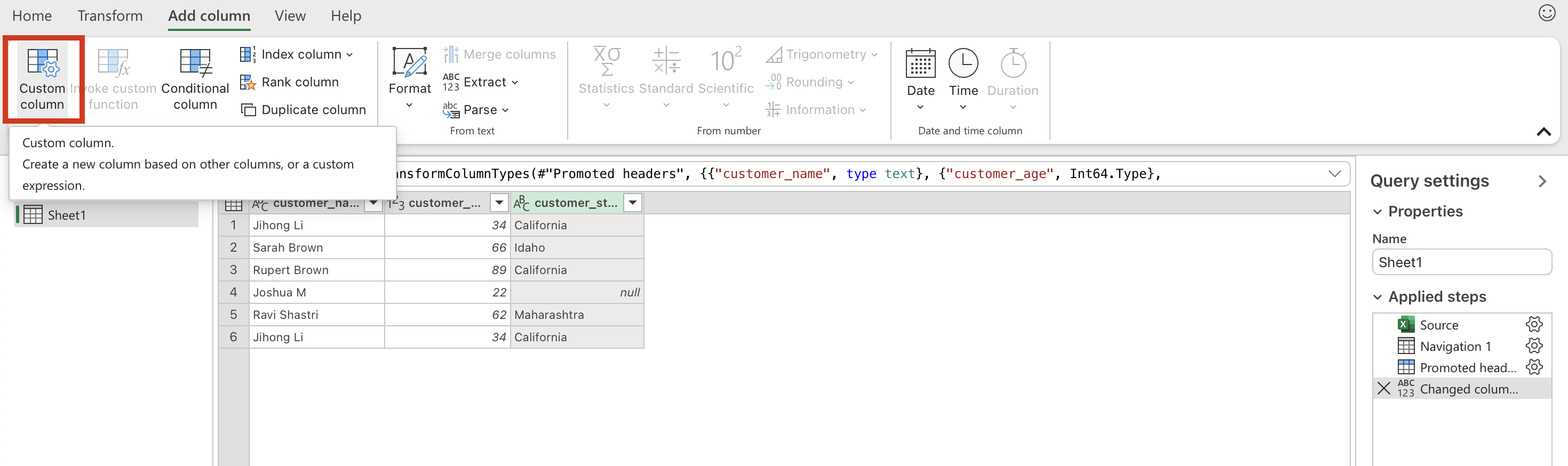
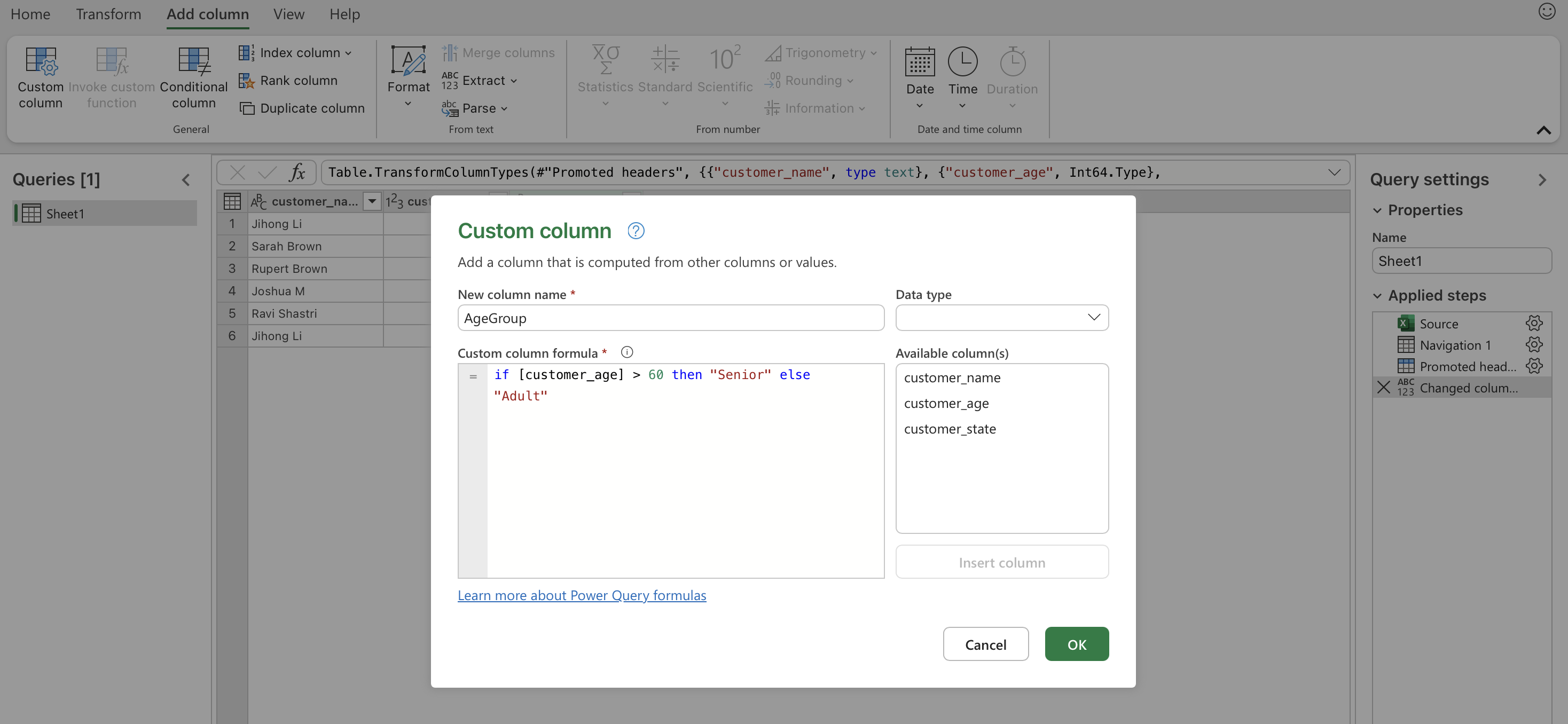
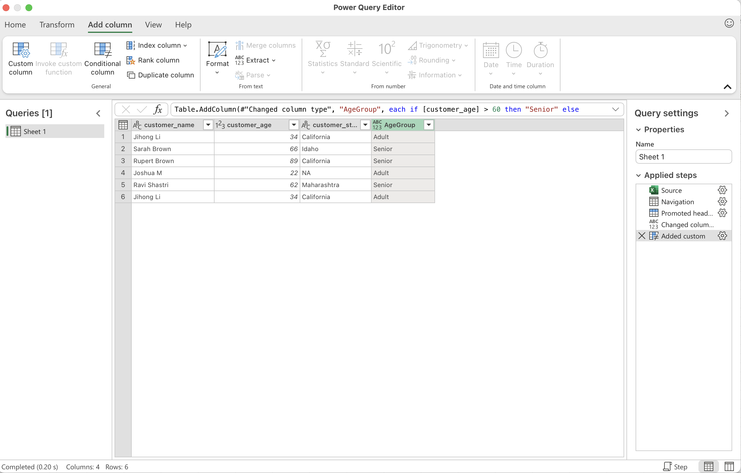
Creating New Columns: Mutate
• Go to the Add Column tab
• Click on Custom Column
• In the formula editor, enter your calculation (e.g., if [customer_age] > 60 then “Senior” else “Adult”)
• Give the new column a name such as AgeGroup and click OK
• Power Query will add this new calculated column to your table
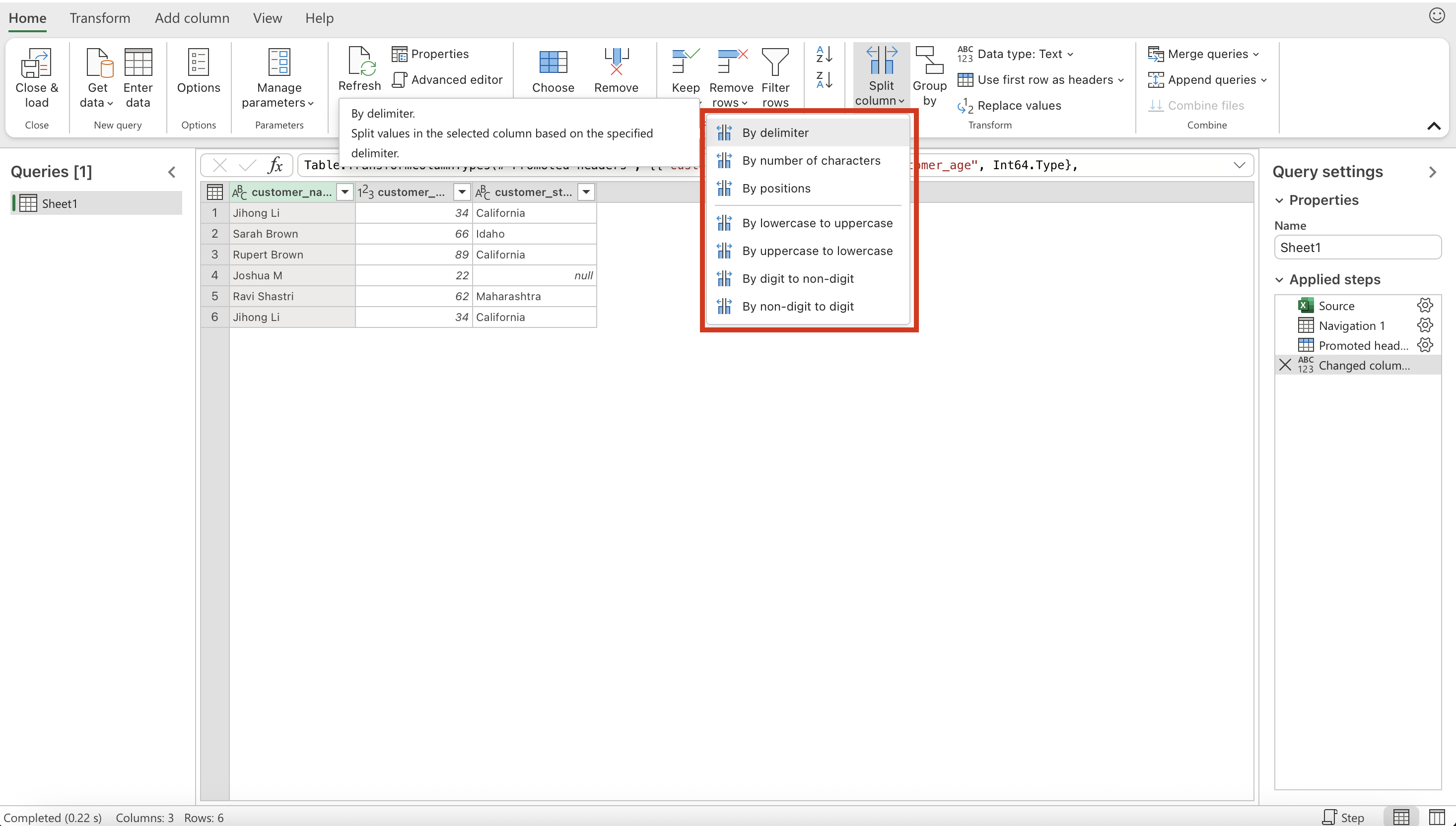
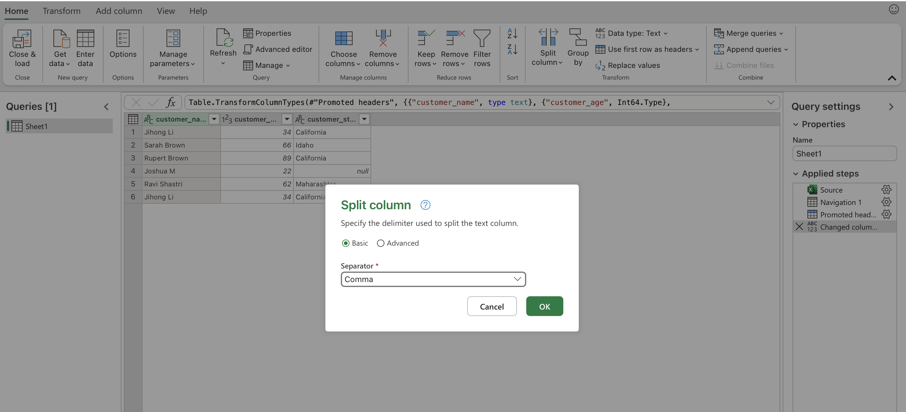
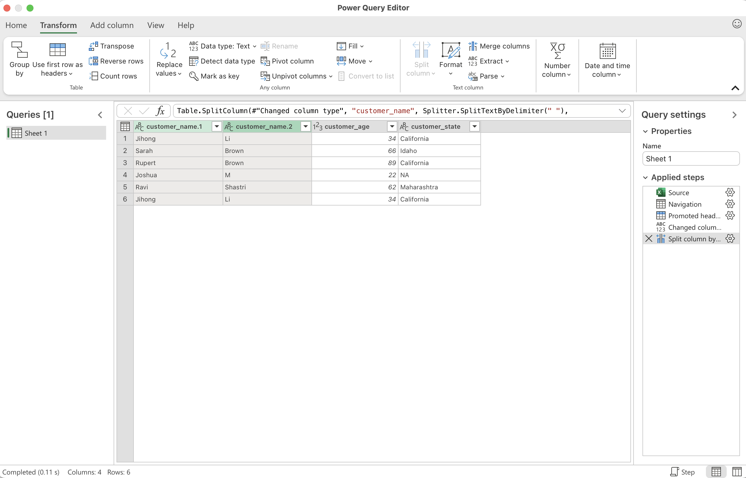
Extracting/Separating Data from Cells: Split Column
• Select the column you want to split (e.g., customer_name)
• Go to the Home tab, click Split Column, and choose By Delimiter (for example, a space ” “)
• Choose whether to split into separate columns or into rows
• Power Query will split names like “Jihong Li” into two columns: Jihong and Li
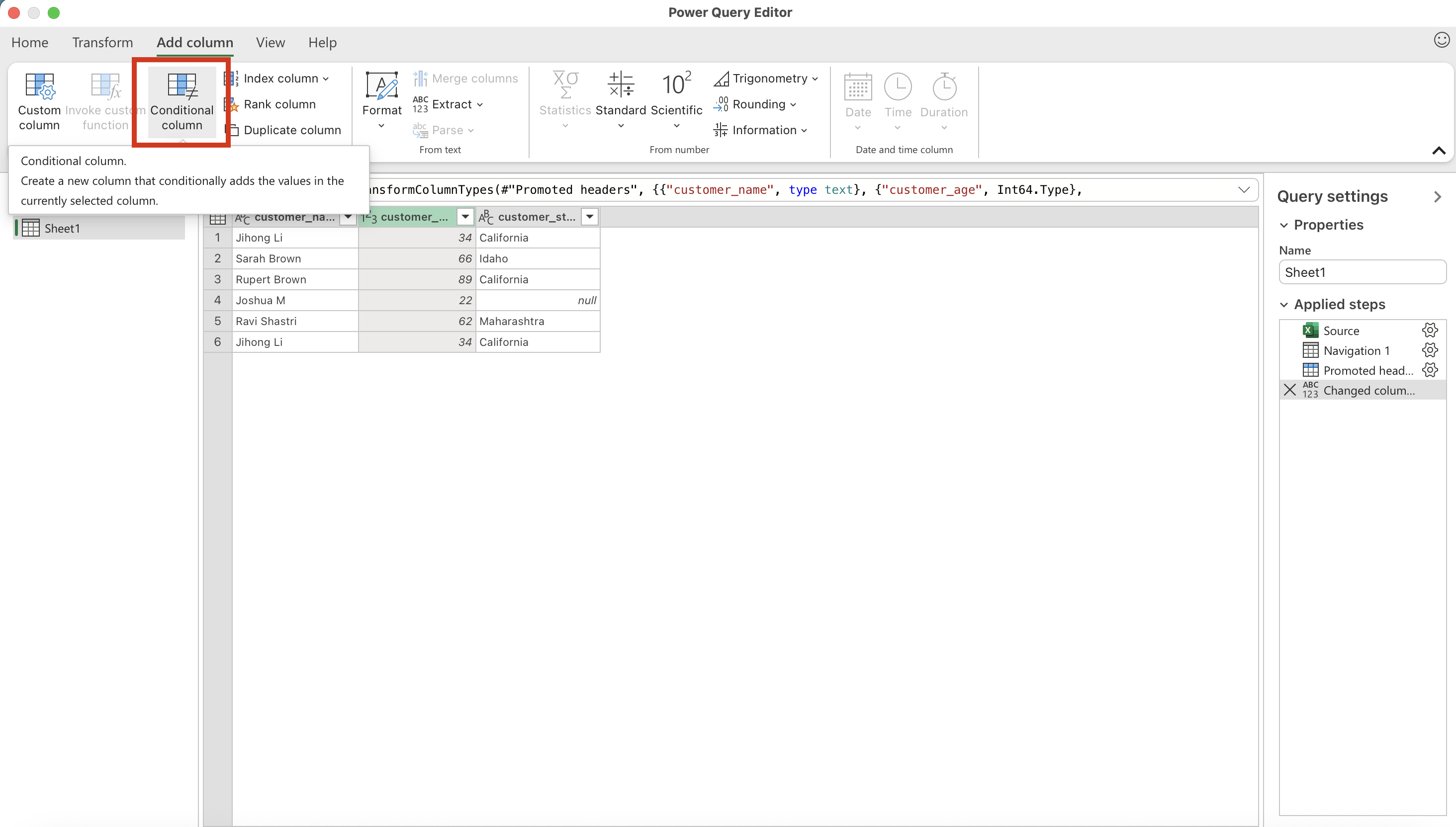
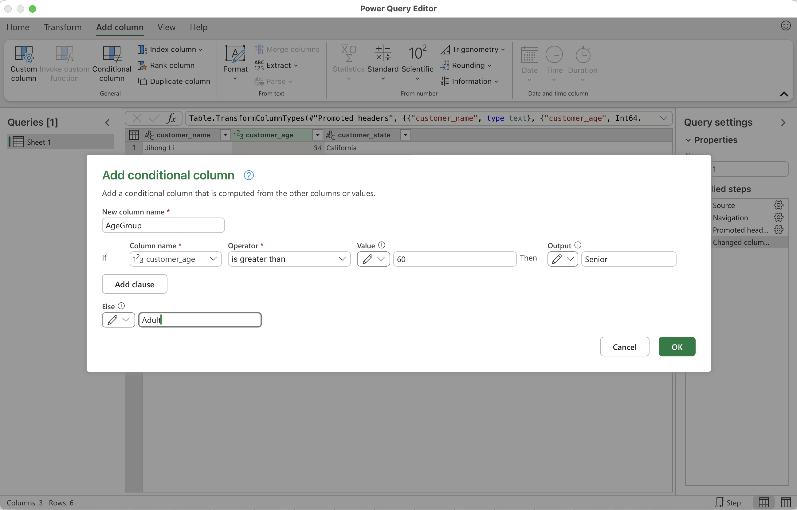
Conditional Cases: Case When
• Select the column you want to base your rule on (e.g., customer_age)
• Go to the Add Column tab and click Conditional Column
• Define your rules (e.g., If [customer_age] ≥ 60 then “Senior” else “Adult”). Click OK
• Power Query will create a new column showing whether each customer is a Senior or Adult
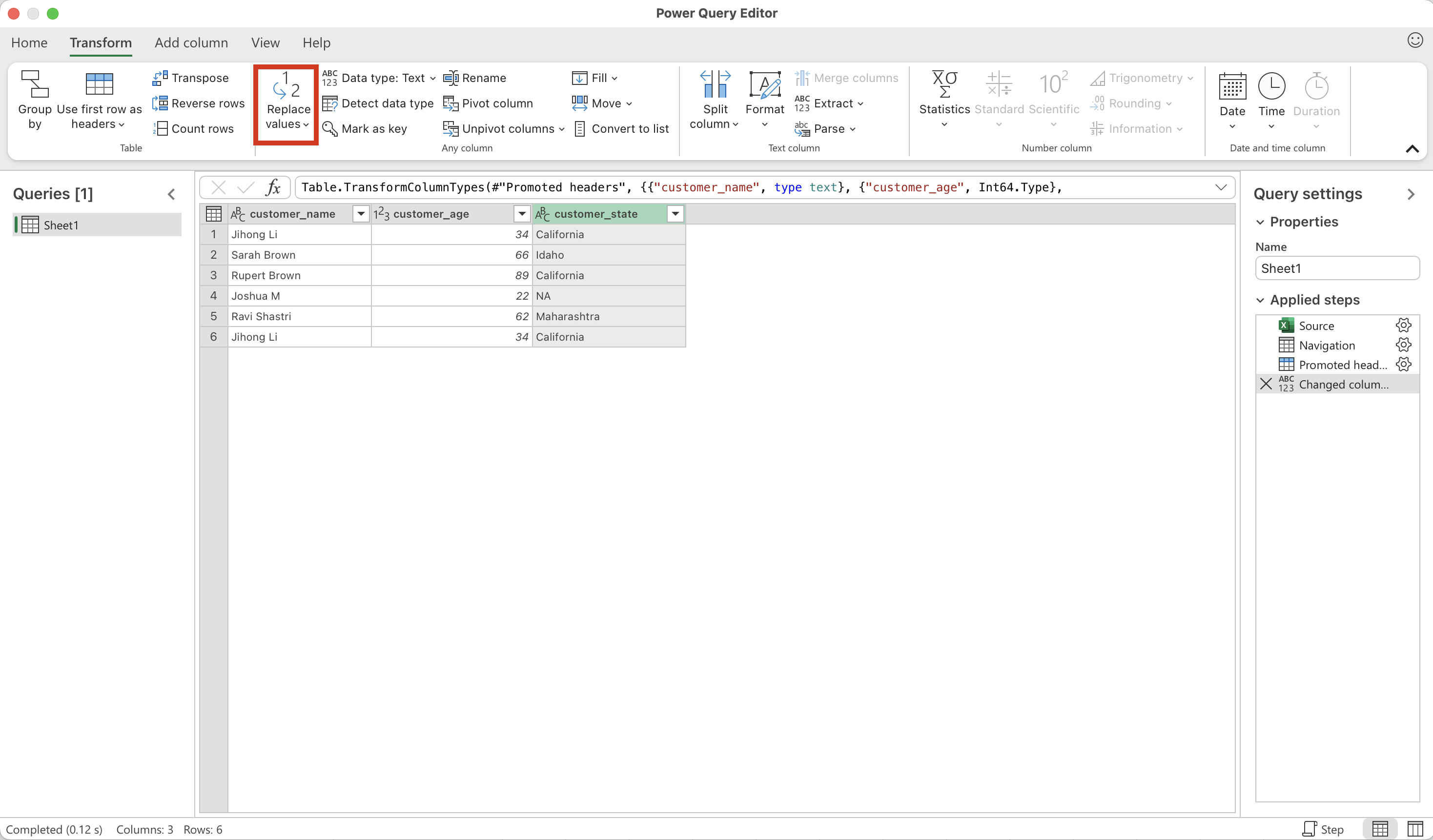
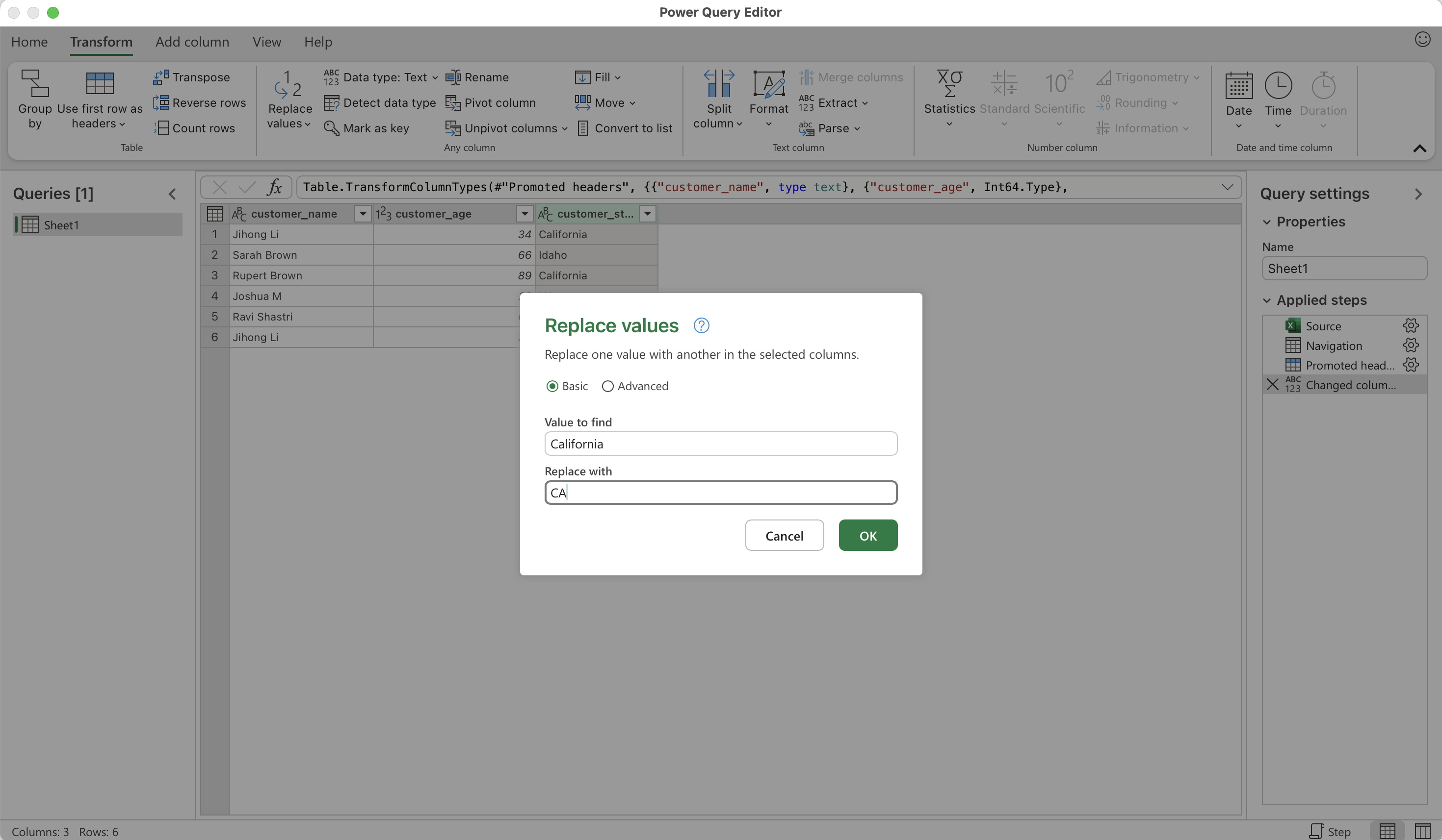
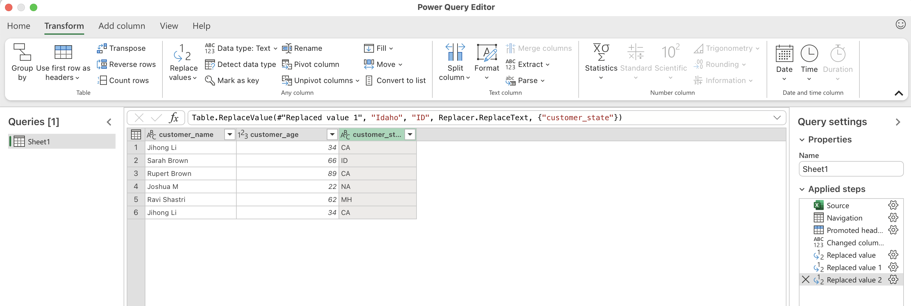
Recode or Lookup Values
Recode
• Select the column where you want to change values
• Go to Transform → Replace Values
• Type in the old value and the new value
• Power Query swaps the old value with the new one inside that column
• Repeat these steps for each value you want to recode
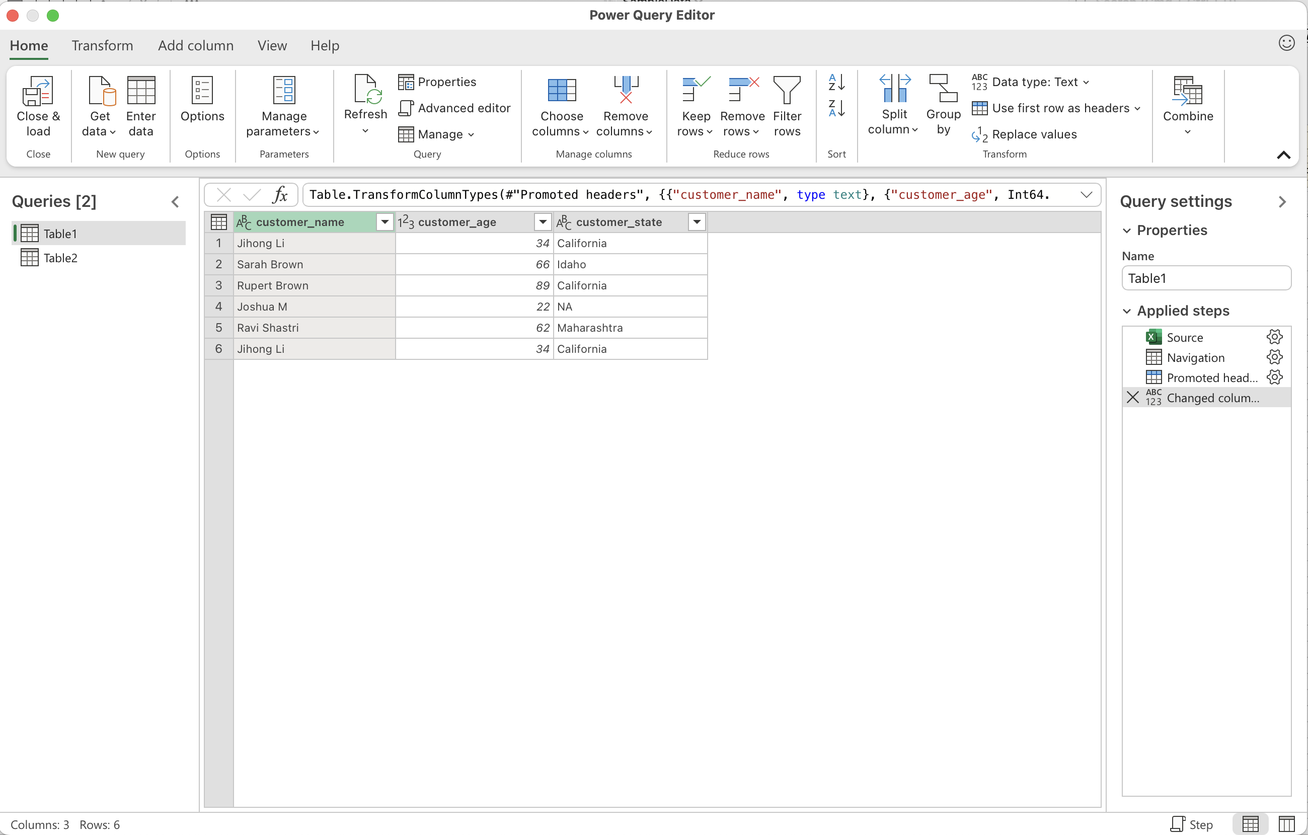
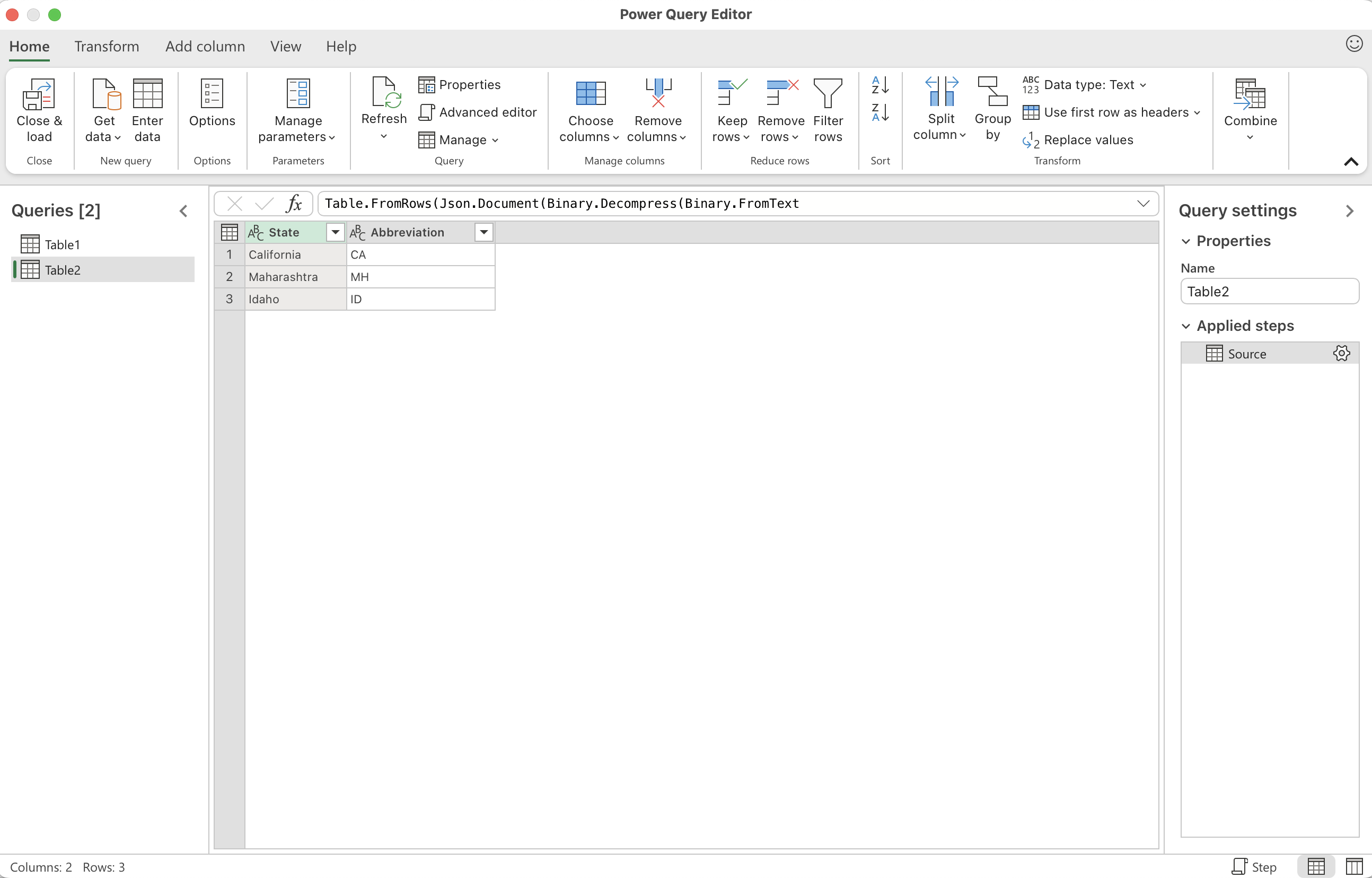
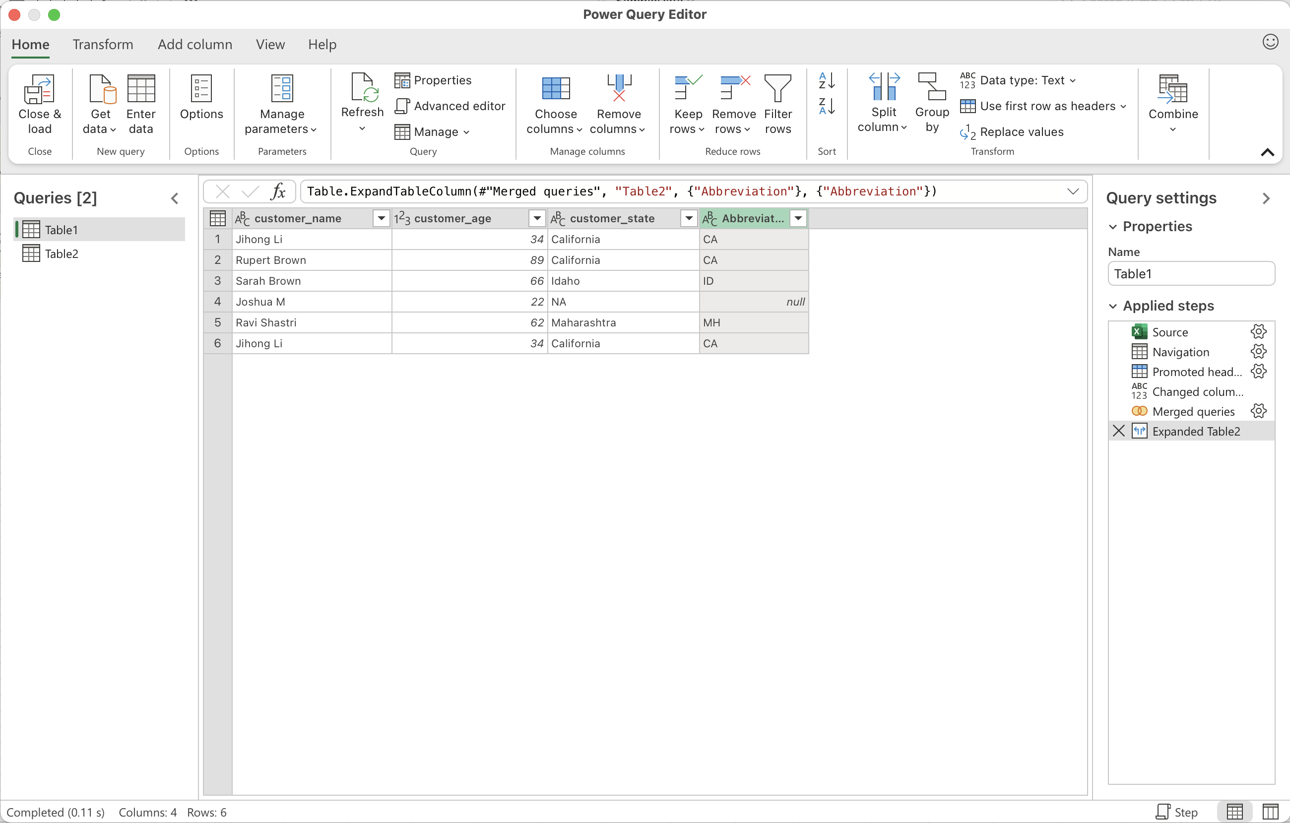
Lookup
• Start with your main table (Table1) that has customer details like customer_name, customer_age, customer_state
• Load the second table (Table2) which has State and Abbreviation values
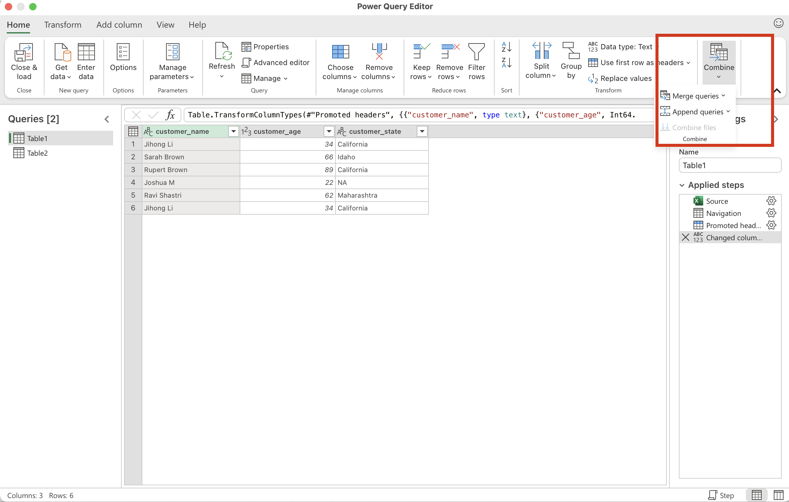
• Go to the Home tab, click Combine, and choose Merge Queries
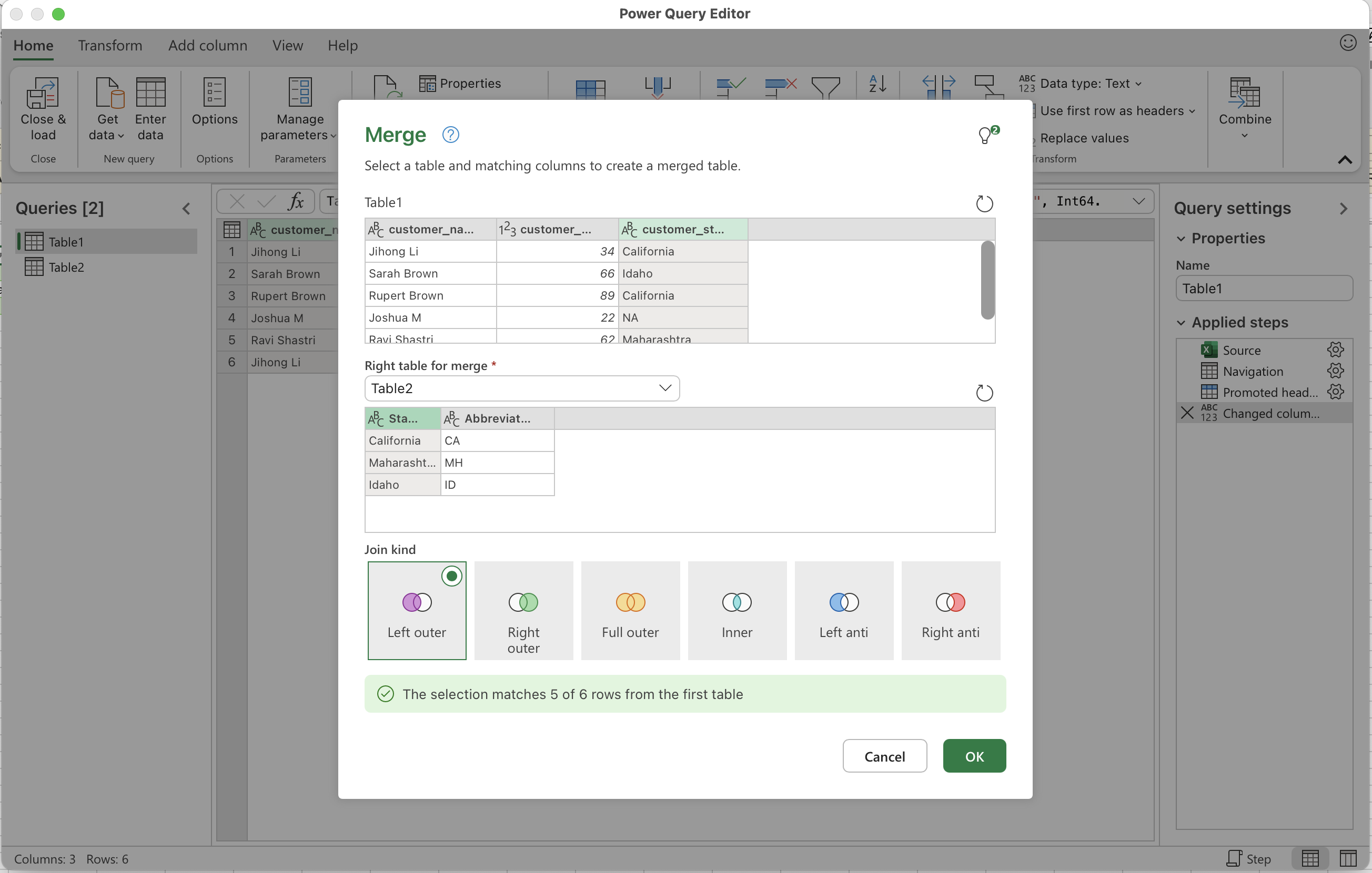
• In the Merge dialog, select customer_state from Table1 and State from Table2 as the matching columns
• Choose the join type and click OK
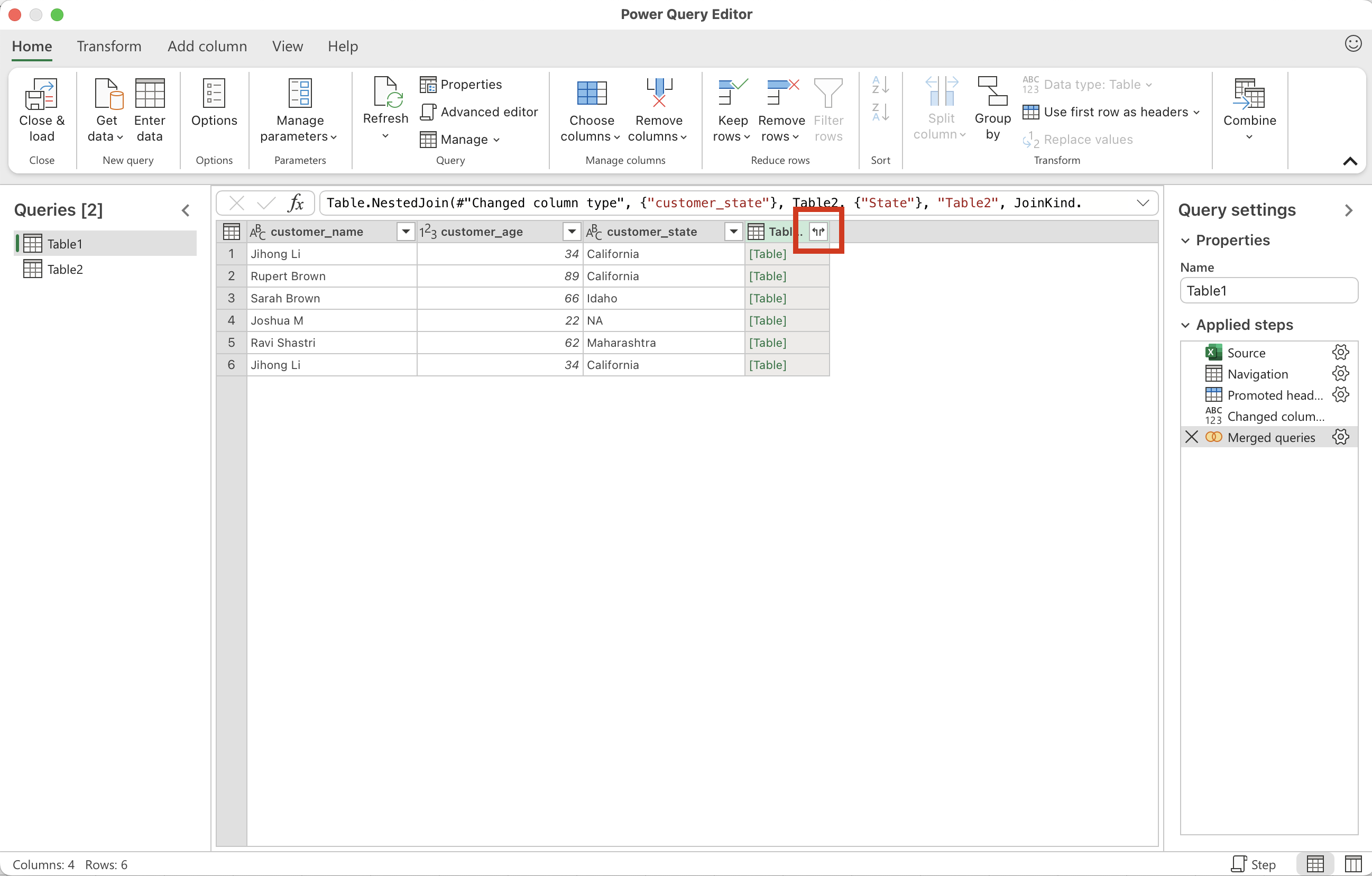
• A new column with [Table] values appears — click the expand icon (two arrows) on top of this column
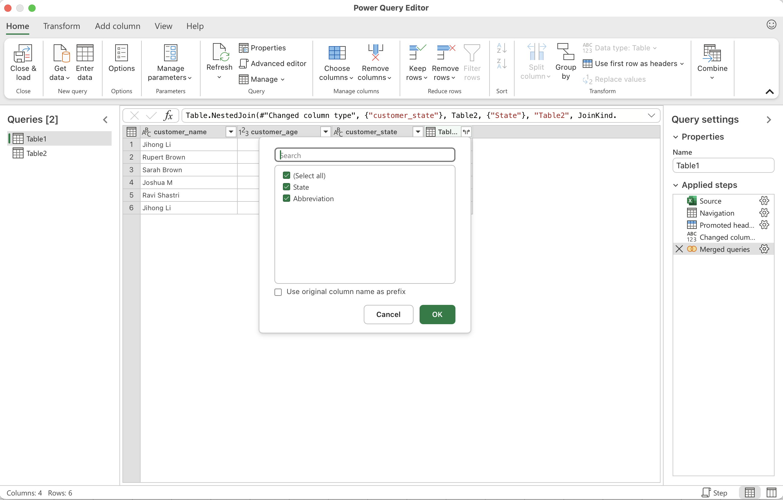
• Select the columns you want to bring in from Table2 (e.g., Abbreviation) and click OK
• Power Query expands the data, showing the new Abbreviation column alongside your original table
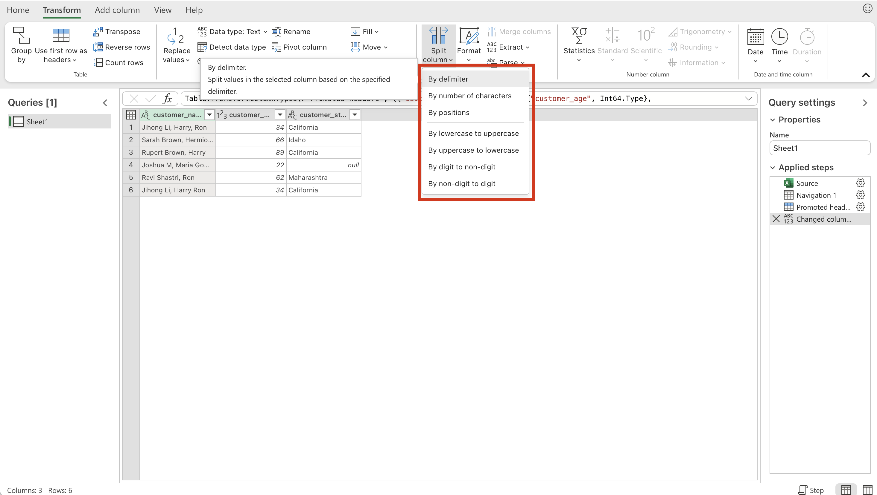
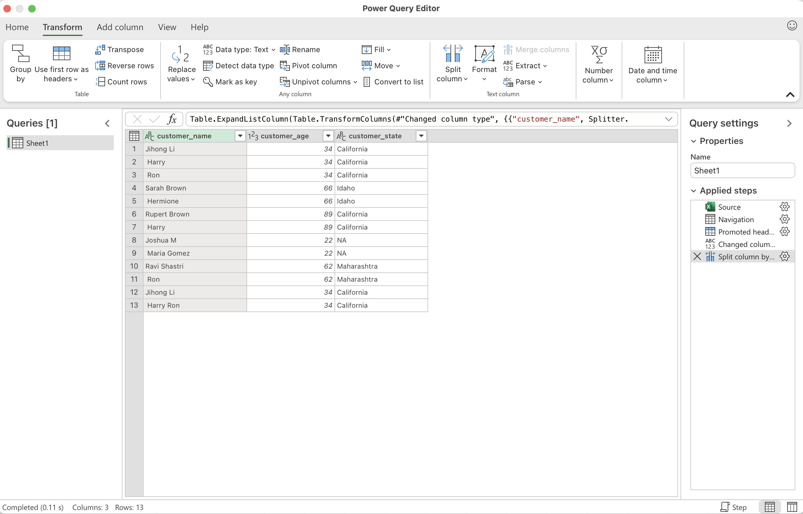
Splitting Lists into Rows: Unnest
• Select the column you want to separate (e.g., customer_name if it contains values like “Jihong Li, Harry, Ron”)
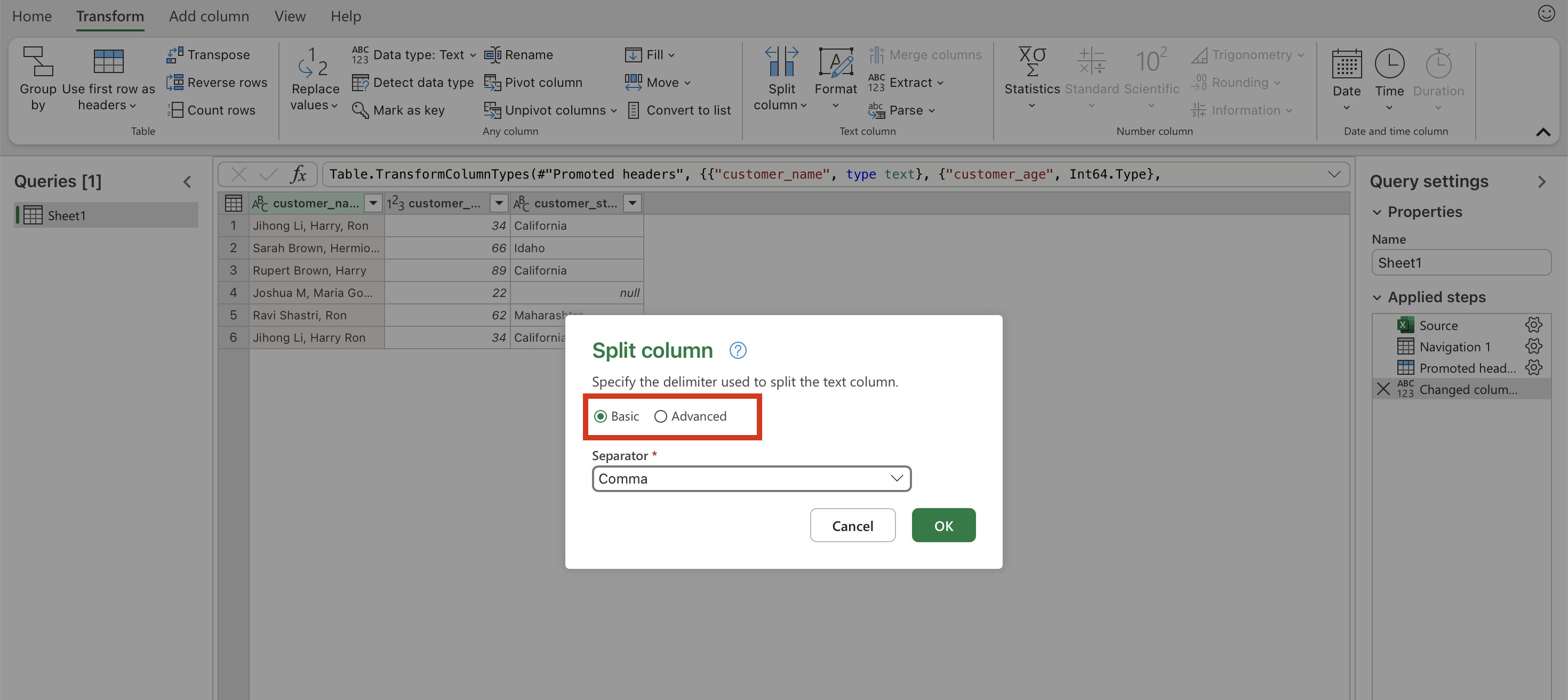
• Go to the Home tab, click Split Column, choose By Delimiter, then select Advanced Options
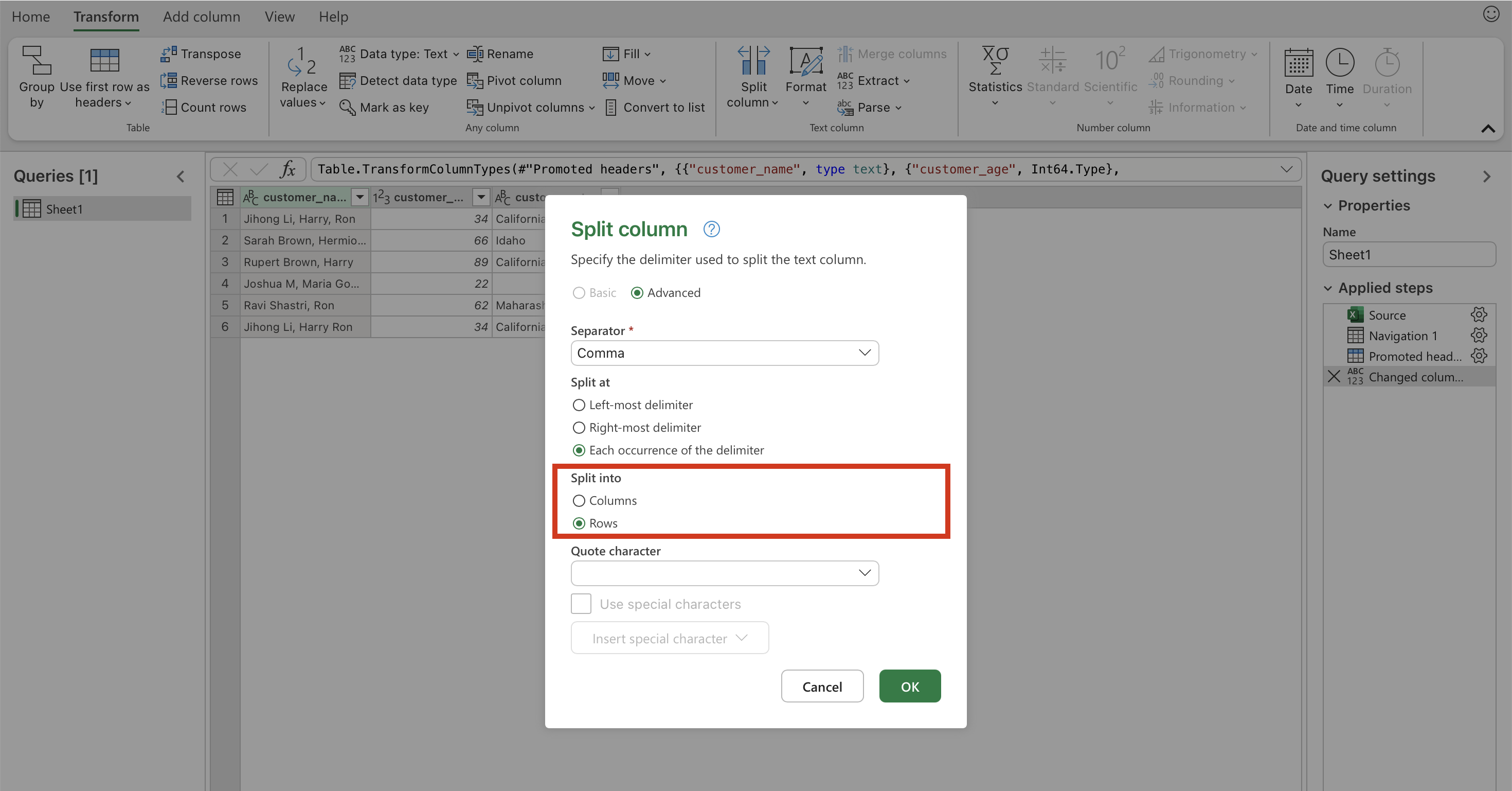
• In the dialog, choose Split into Rows instead of columns
• Power Query will expand the value “Jihong L, Harry, Ron” into three rows
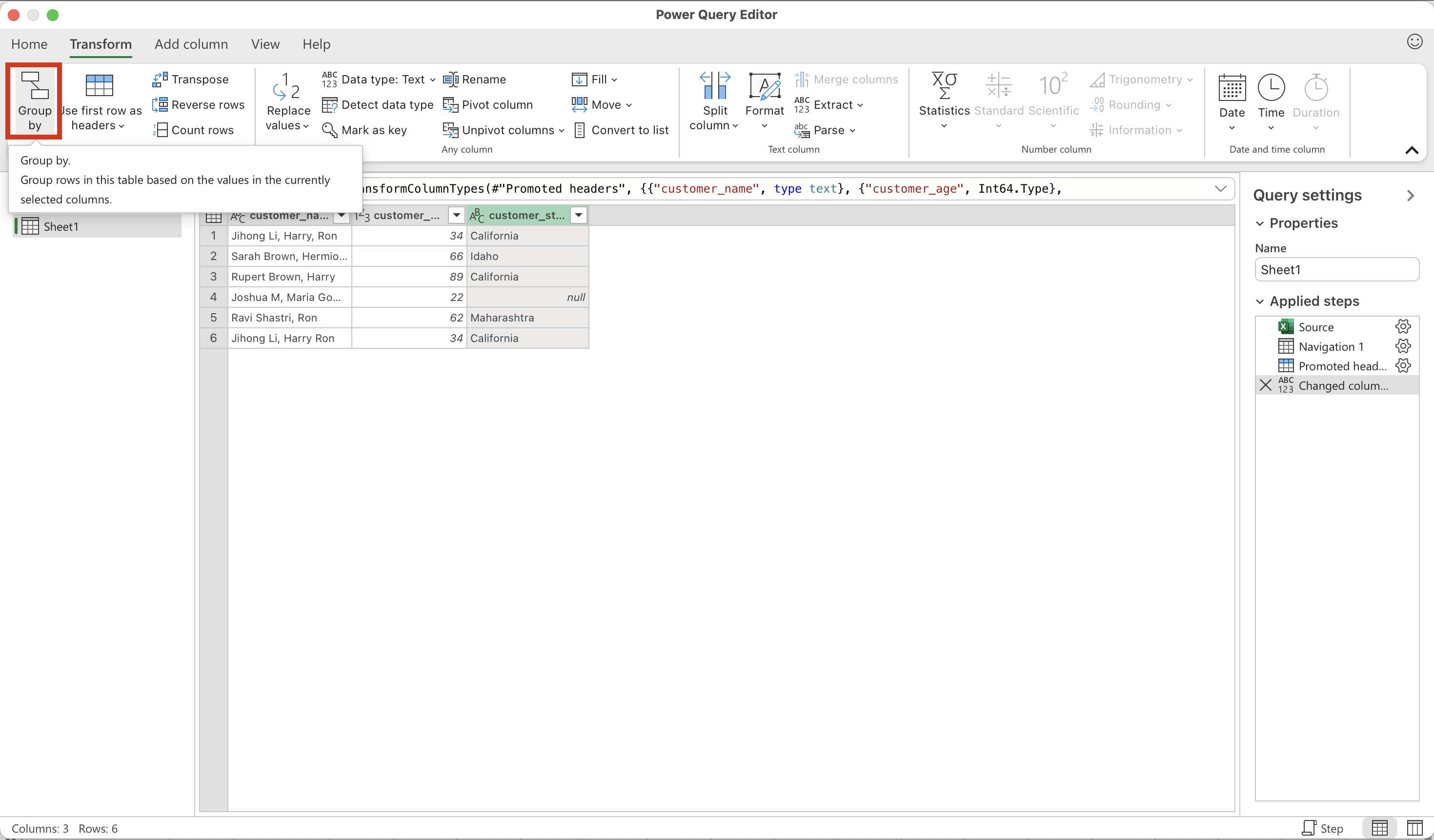
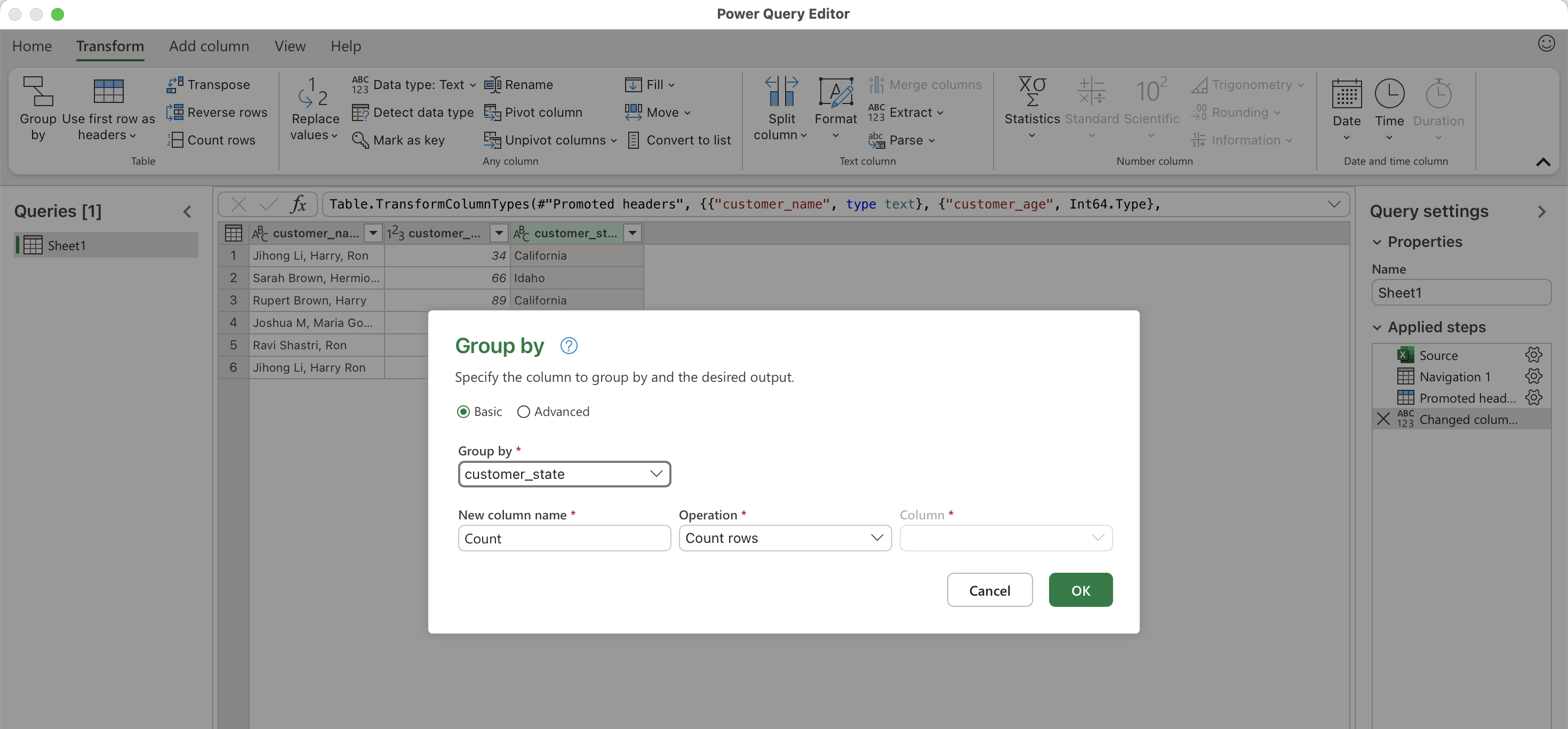
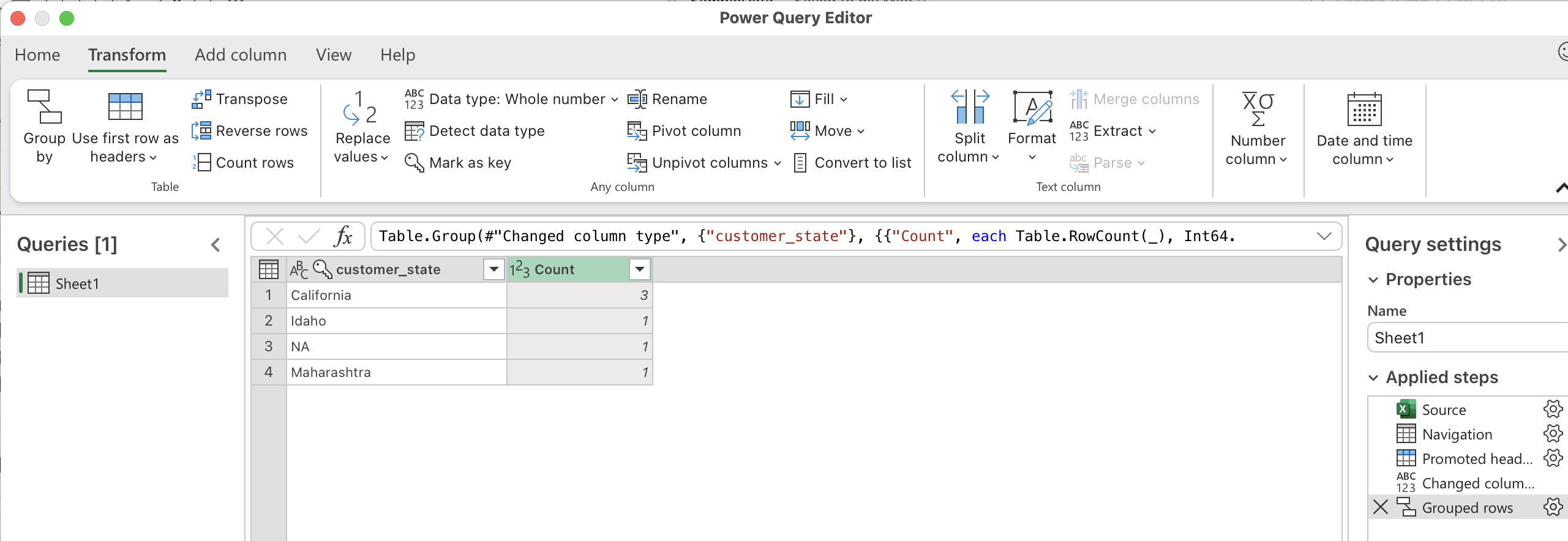
Grouping and Aggregating: Group By & Summarize
• Go to the Home tab and click Group By
• Choose the column you want to group on (e.g., customer_state)
• In the Operations box, pick the aggregation you need (e.g., Count of customer_name)
• Power Query will return one row per state, showing how many customers belong to each state
Reshaping Data: Pivot/Unpivot
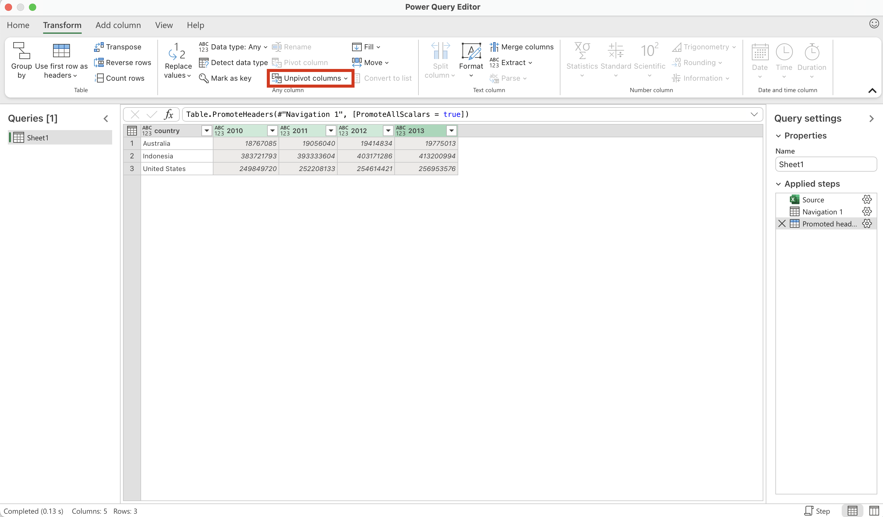
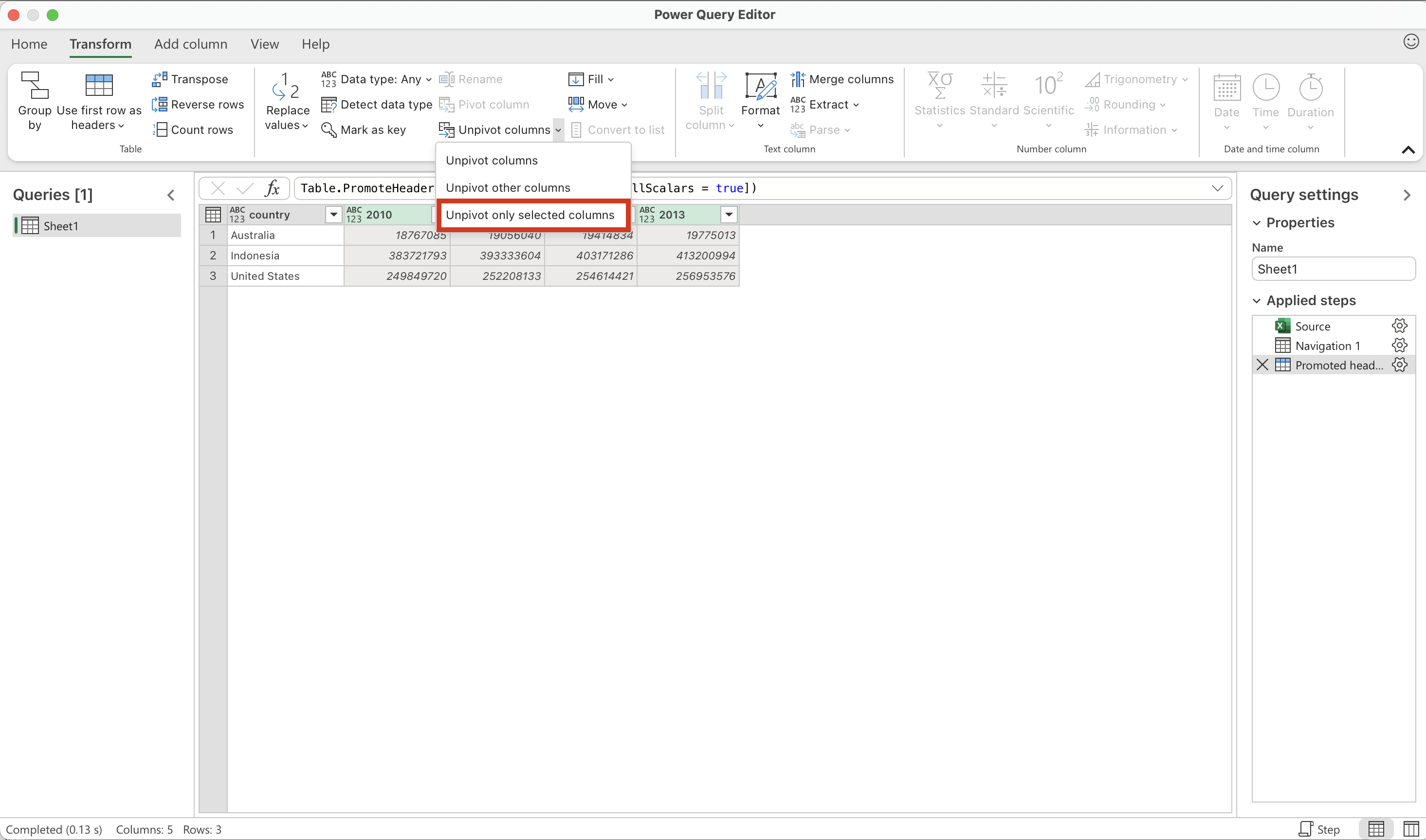
Unpivot (Wide → Long):
• Select the identifier column you want to keep (e.g., country)
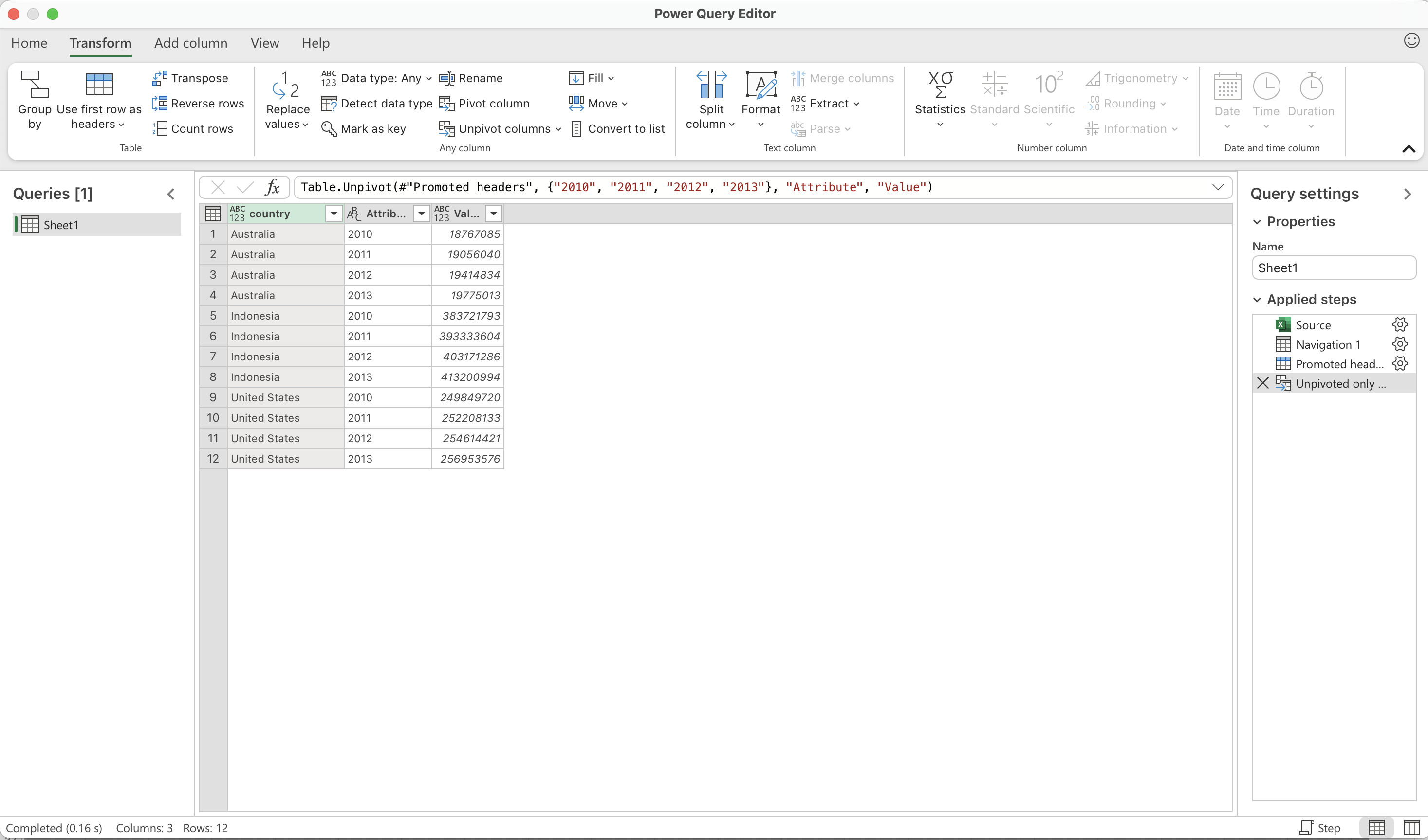
• Go to the Transform tab, click Unpivot Columns, and choose Unpivot Only Selected Columns (e.g., 2010, 2011, 2012, 2013)
• Power Query will create two new columns: Attribute (Year) and Value (Population)
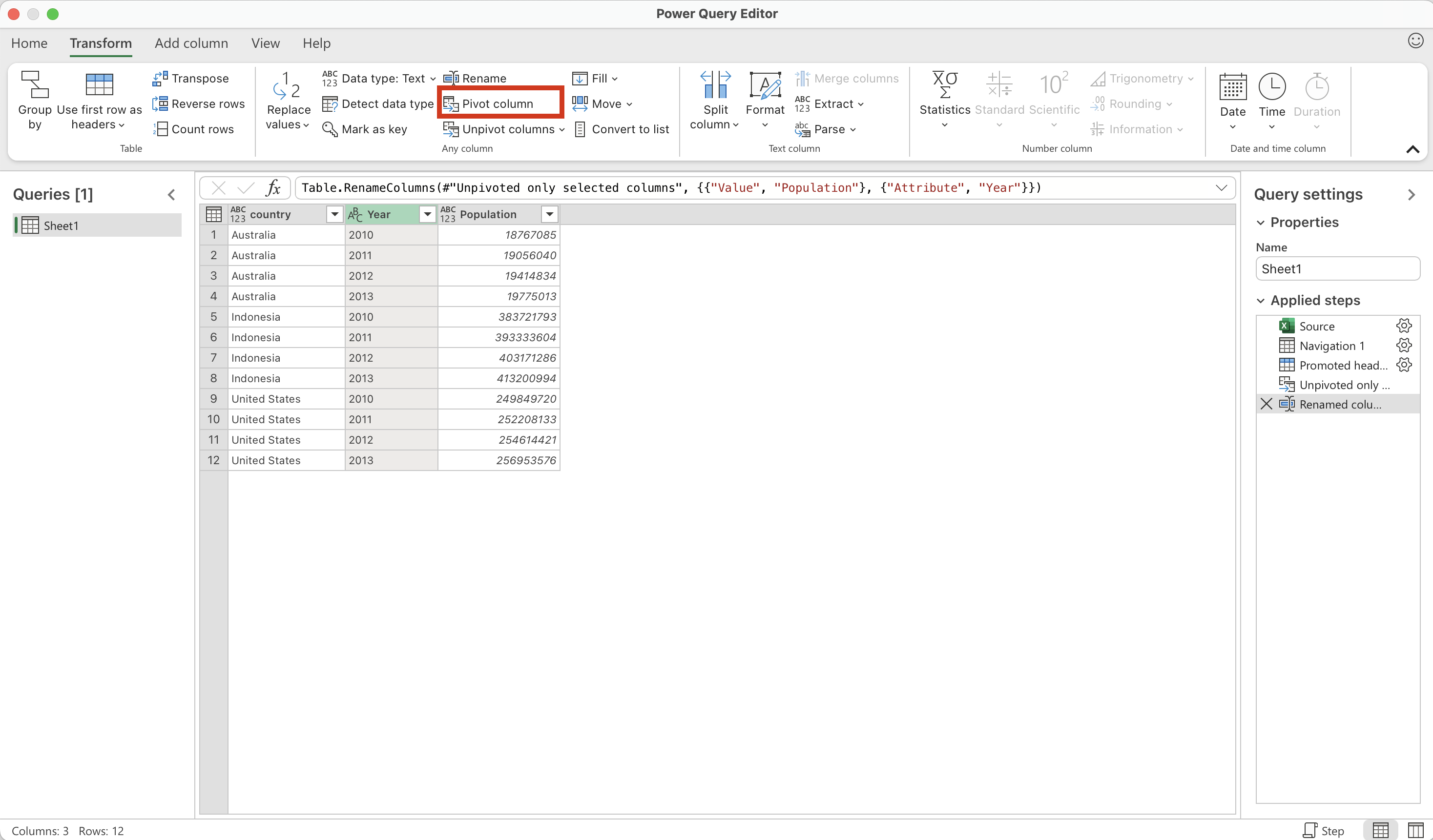
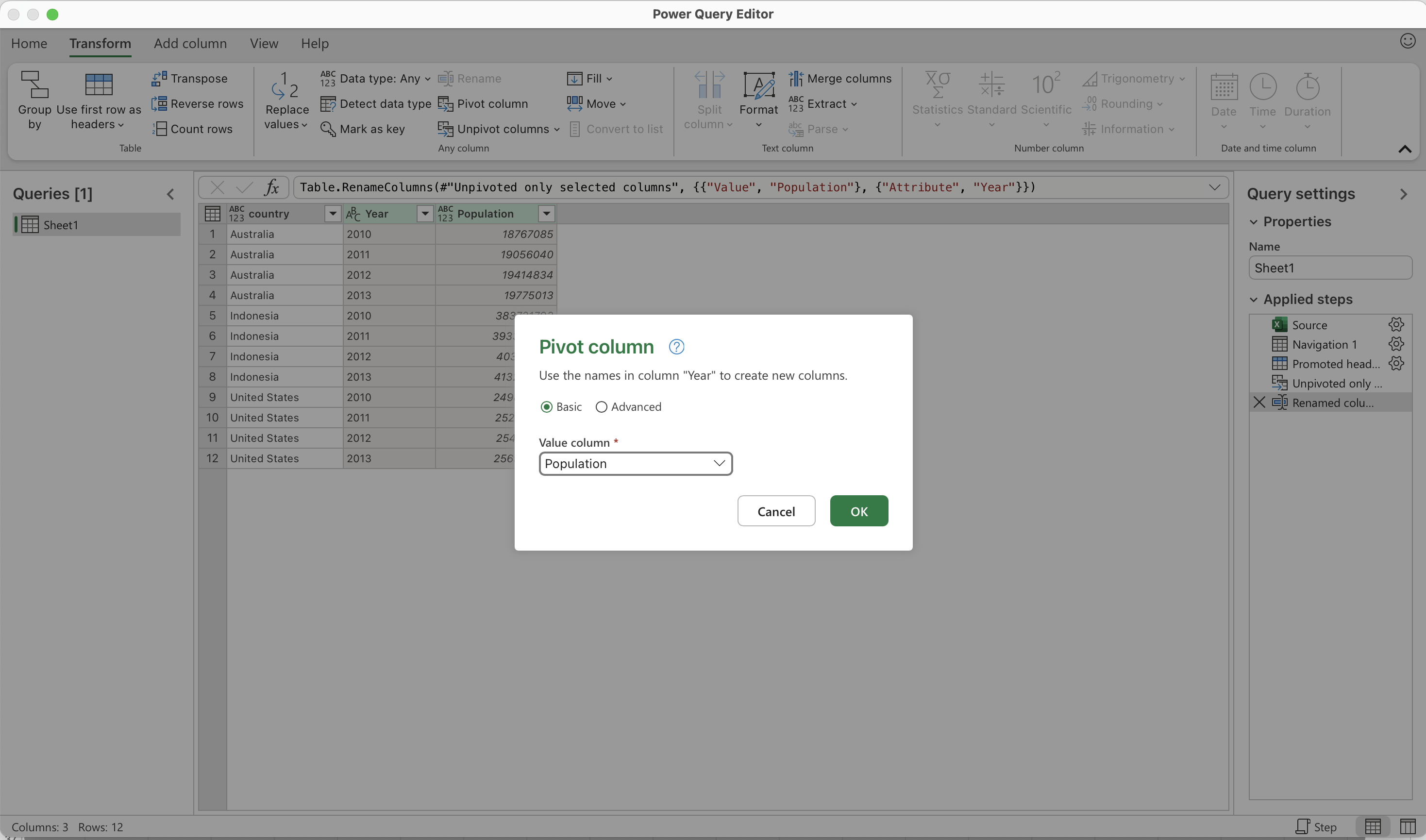
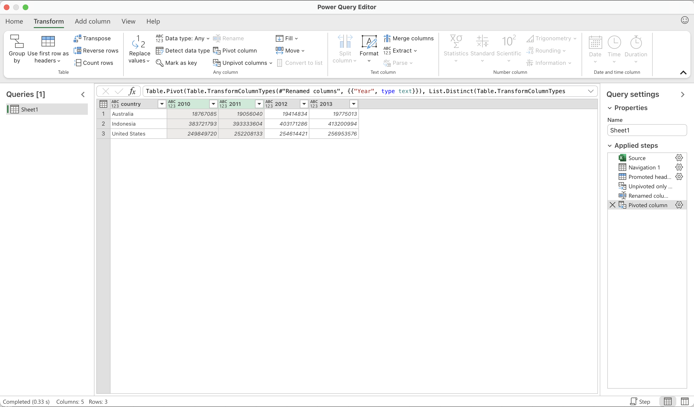
Pivot (Long → Wide):
• Pick the column whose values you want to turn into headers (for example, Year)
• Go to the Transform tab and choose Pivot Column
• Select the column that has the numbers or data you want to fill in (for example, Population)
• Power Query will rearrange the table into wide format, creating separate columns like 2010, 2011, 2012, 2013
Advantages/Disadvantages of Power Query
The main difference is that Pandas, R, and SQL need you to write code; Power Query lets you do the same transformations just by clicking and selecting options. It keeps track of all the steps for you, so you don’t have to remember commands. Since it’s built right into Excel, it’s very handy for quickly cleaning and organizing data; it is also used in other Microsoft products, such as Power BI and the Sharepoint ecosystem.
Underneath it does write code (in a language called M), although my sense is that people rarely examine that underlying code.
A downside of Power Query is that it is harder to share and collaborate using version control like git or github.