Excel Worksheet Transforms

Note

Before starting on Excel, do the SQL Warm-up: Music Festival. It introduces the music festival database that we will also use in Excel.

The screenshots on this page use other data, but the “Try it” boxes use the music festival data. Download music_festival.xlsx. It has three worksheets, performances, venues and bands, with the same columns as the SQL tables.

Excel is a powerful tool; you can do many of the same things we’ve been doing in SQL in Excel. I used to claim that there were things that you couldn’t do, but I was always shown to be wrong by someone!

Having said that, Excel does things differently than SQL and definitely has trouble with lots of data. That is for two reasons:

First, Excel always shows all the data, so it all has to be in the computer’s active memory (RAM), whereas SQL keeps things on disk. That can make things like scrolling through the data slow and laggy.

Second, Excel doesn’t have some of the advanced algorithms that make large joins very efficient.

Excel and tabular data

Excel arranges data in rows and columns, just like SQL. However, the columns are not like fields in SQL in that they are not “strongly typed” (meaning that you could have regular text in a column right above a date or a number) and the structure of columns and rows is not tightly enforced (you could have one row with 5 columns and the next row having only 3, or a “table” with lots of footnotes or even multiple tables per worksheet).

In fact it’s better to think of Excel in its default state as closer to a word processor (like Word) using fancy tables (which is not to say that you can’t change the defaults to enforce datatypes, just that the defaults are not like that).

Excel also doesn’t have a strong concept of a row that groups the elements together. So it’s possible to end up moving data in a field to a different row, something that sometimes happens accidentally. In a sheet that has people, their names and their ages, you might end up swapping one person’s “age” with another person, not typically something you want to do!

Excel allows multiple “Worksheets.” These are used like tabs in a browser; they can hold separate data, but can also hold user interface elements, like graphs or even laid-out text. So you can sometimes think of worksheets as like different tables in SQL, but keep in mind that while they can work like that, they don’t always.

Almost all we’re going to explore in Excel relies on having data set up as tabular data, very similar to tables in SQL: columns (with headers) and rows of data, each row representing a different record (or instance of an Entity).

Sorting rows: Sort

When you have an Excel sheet set up with data in columns and rows, you can sort and filter, just as we did in SQL.

Sorting requires selecting the data first. Be careful here as it’s possible to select only a subset of the data, leaving parts of it unsorted (if you leave off rows), or breaking up rows (if you leave off columns). I typically either select the whole sheet (clicking in the upper left hand corner of the worksheet, see the little triangle thing?) or select the columns I want to sort by clicking on the column headers and dragging across.

You can then choose Data -> Sort from the menus. Be sure to check “My list has headers”. The sort panel looks like this (I’ve clicked in the Column column). You can sort by multiple columns (just like ORDER BY two fields) by clicking the + symbol and adding a second sort condition.

Try it: sort

On bands, sort by fee, largest first. What is at the top? (Remember the test rows from the SQL warm-up.)
On performances, sort by venue_id and then by start. That gives the running order for each stage, like ORDER BY venue_id, start.

Excluding rows: Filter

Filtering is Excel’s equivalent of SQL’s WHERE (or filter in R): it excludes rows, such as WHERE username = 'james'. Unlike WHERE, Excel filters hide rows rather than removing them.

There are many options for filtering, but an immediately useful one is to turn filtering on by choosing Data -> Filter from the menus. That creates a drop down on the first row (headers). Data -> Advanced Filters can copy the result of filtering to another sheet.

When you have a filter set the tiny icon on the table header changes and the row numbers are highlighted in blue (indicating hidden rows). Below I have two filters set (one on username, one on actiontype), the equivalent of WHERE username = 'james' AND actiontype = 'post'.

Try it: filter

On performances, filter venue_id to 1 (that’s AMD). How many performances were there? Clear the filter afterwards.
On bands, use a Number Filter to show bands with a fee greater than 2000. How many are there, and which of them look like test data?

New columns: formulas

Excel’s strength is in calculations, doing things like adding up columns of numbers or multiplying one cell by the contents of another. This reflects Excel’s accounting heritage. Using these features we can achieve things similar to both aggregate functions in SQL (COUNT, SUM and AVG) and math in SELECT that creates new columns (like mutate in R).

Calculations are done via formulas which are indicated by typing text into a cell starting with the = sign. Unlike SQL, formulas refer to locations on the worksheet using column letters and row numbers, not headers (column names). Thus A2 refers to the cell in the first column, but in the second row. We enter a formula into a cell where we want the answer to appear, for example we might have the number 7 in A1 and the number 7 in B1 and want to put the result in B3. In cell B3 we’d write: = A1 + B1

Here we are adding together 7 (A1) and 7 (B1) and putting the answer into B3. If we later change the value in A1 or B1, then the formula will recalculate, changing the result in B3.

If we want to do a calculation to create a new column for a tabular (“table-like”) sheet with rows and columns, we locate a new empty column (perhaps using insert) and then write the formula into the top cell, and copy the formula down the page. Roughly speaking this is the equivalent of:

SELECT *,
       ticket_price * tickets_sold AS total_revenue
FROM shows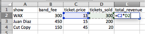

Here I’ve clicked in E2 and typed = (indicating that I want to enter a formula). Then I clicked in C2 (making it highlight blue and the click enters C2 into the formula). Then I type * (for multiply) and then click D2. When I press enter, the formula will calculate the total revenue (here tickets are all the same price).

To do the same for Juan Diaz, we’ll need to have a similar, but slightly different, formula in the cell E3. Rather than having the number 2 in the formula we’ll have the number 3. Happily, Excel understands this and thinks about where the formula is being pasted from and where it is pasted to, and changes the numbers accordingly. So if you select E2, choose copy, and then paste into E3, hit return, then double-click in E3, you’ll see that the 2s in the formula changed to 3s.

There are many ways to copy a formula down a full column. One is by dragging down the + symbol that appears when you click a cell and hover over its bottom right corner (the mouse cursor doesn’t show up in this screen shot, but it will appear right on top of the blue square):

If you then click and drag down the column, Excel will “fill down” and copy the formula, again adjusting the row numbers so that each copy of the formula refers to the right row. Another way to do this is to double-click the little handle that you pulled down; if the sheet is organized like a table, then this will fill the contents of that cell down the column. Handy!

Sometimes you don’t want Excel to adjust a reference when you copy a formula, for example when you want to multiply a whole column by the value in a single cell. Then you put a $ in front of the part you want to keep fixed. Below, the formula in C4 is =B4*$D$1. Copied down to C5 it becomes =B5*$D$1: the B4 moved with the row, but $D$1 stayed put. You can fix just the column ($D1) or just the row (D$1).

Try it: new columns

On performances, type length in F1 and =C2-B2 in F2, then copy it down. Excel stores datetimes as numbers of days, so the answer looks odd at first: use Format Cells and choose the time format h:mm. How long was the longest performance?
On bands, type 1.1 in F1 (a 10% raise). Type new_fee in D1 and =C2*$F$1 in D2, then copy it down. Change F1 to 1.2 and watch the column change.

Aggregates: SUM

You can produce totals of columns, like using SUM() in SQL. In fact it’s the same function name:

Here I’ve clicked in E5 and typed =SUM(. To indicate what cells you’d like to add up, you have to enter a range, which is done as the name of the starting cell, then a colon, then the name of the ending cell. You can get this by clicking and dragging over the cells (then typing close parens).

Try it: SUM

On bands, add up the fee column. Keep the answer: we’ll come back to it after the lookup below.

Recode/lookup: XLOOKUP

Excel worksheets don’t have a JOIN command, but a lookup formula does something very similar: for each row, find the matching row in another table and bring back a value from it. (Power Query, covered in Excel Power Query, does have a real join, called Merge Queries.) Lookup formulas can be slow with lots of data, but you will see them everywhere in spreadsheets, especially from collaborators who work only in Excel.

Here we have some data from a web log, showing a datetime, the name of a user and the sort of action that the user took: either join for when they joined the site (nothing to do with a database join!), or post for when they posted something on the site.

datetime	user_name	action_type
2011-04-03	Matthew Reyes	post
2011-04-07	Stephen Lewis	join
2011-04-09	Frank Sims	post
…	…	…

You want to add a column saying whether the user in that row is a “manager” or “volunteer”. You could do this by hand, but with many, many rows of data that’s not a great idea. Instead, another worksheet holds a table with the related data about each user:

user_type	user_name
manager	Matthew Reyes
volunteer	Lillian Turner
volunteer	Frank Sims
…	…

We want to match on user_name and bring the user_type column over to the log. Users who aren’t in the second table (like Stephen Lewis) are ordinary users, so they get “user”.

datetime	user_name	action_type	user_type
2011-04-03	Matthew Reyes	post	manager
2011-04-07	Stephen Lewis	join	user
2011-04-09	Frank Sims	post	volunteer
…	…	…	…

In SQL this is a LEFT JOIN, matching on a text column rather than an id column, followed by filling in the NULLs for users with no match:

SELECT log_data.*,
       user_types.user_type
FROM log_data
  LEFT JOIN user_types
    ON log_data.user_name = user_types.user_name

Data for the lookup

Download this Excel file, which has the two tables on two worksheets, log_data and user_types. If you want to practice getting csv files into Excel, you can get the original files here:

log_data.csv - shows events by users
user_types.csv - gives a user type label for some users

Caution

The formulas below refer to the worksheets by name (user_types!). When Excel opens a csv file it names the worksheet after the file (without .csv). If your worksheets have different names, change the formulas to match. You’ll know this has happened if Excel asks you to find a file called user_types.

On the user_types worksheet the user type is in column A and the user name in column B:

	A	B
1	user_type	user_name
2	manager	Matthew Reyes
3	volunteer	Lillian Turner
…	…	…
7	volunteer	Frank Sims

The XLOOKUP formula

On the log_data worksheet, type user_type as the header in D1, then put this formula in D2:

=XLOOKUP($B2, user_types!$B$2:$B$7, user_types!$A$2:$A$7, "user")

XLOOKUP takes four things:

what to look for: the user name in this row ($B2)
where to look for it: the user names on the user_types worksheet (user_types!$B$2:$B$7)
what to bring back: the user types, in the same rows (user_types!$A$2:$A$7)
what to use if there is no match: "user"

Excel works the formula out step by step. For row 2, it replaces each reference with what is in those cells, then looks for the name in the first list and returns the item at the same position in the second list. Matthew Reyes is 1st in the list of names, so the answer is the 1st item in the list of user types (press Step or Play). The lists are written Python style here; Excel itself writes them with curly braces.

XLOOKUP($B2,user_types!$B$2:$B$7,user_types!$A$2:$A$7,"user")
XLOOKUP("Matthew Reyes",user_types!$B$2:$B$7,user_types!$A$2:$A$7,"user")
XLOOKUP("Matthew Reyes",["Matthew Reyes", …, "Frank Sims"],user_types!$A$2:$A$7,"user")
XLOOKUP("Matthew Reyes",["Matthew Reyes", …, "Frank Sims"],["manager", …, "volunteer"],"user")
"manager"

For Stephen Lewis there is no match, so the formula returns "user". Without that fourth part, Excel shows #N/A (“Not Available”), its version of the NULL that a LEFT JOIN leaves when there is no match.

Now copy the formula down the column (double-click the fill handle). The $ signs matter here: $B2 lets the row change as you copy down, while $B$2:$B$7 and $A$2:$A$7 stay fixed, so every row searches the whole user_types table.

Notice that the column we bring back (A) is to the left of the column we search (B). XLOOKUP doesn’t mind; the older VLOOKUP can only bring back columns to the right of the one it searches.

Try it: XLOOKUP with the festival data

The join conditions from the SQL warm-up tell you how to write each lookup. For venues.id = performances.venue_id, the _id column is what to look for, and the id column is where to look for it.

On performances, type venue_name in F1 and put this in F2, then copy it down:
```
=XLOOKUP($D2, venues!$A$2:$A$11, venues!$B$2:$B$11)
```
Add band_name in G and fee in H, looking up band_id (column E) in bands. The bands data runs from row 2 to row 134.
Filter venue_name to AMD and sort by fee, largest first. Which band had the highest fee? Check it against exercise 3 in the SQL warm-up.
Add up your new fee column. That is what the festival actually paid its bands. Why is it so different from the total on bands?

Try it: XLOOKUP as a LEFT JOIN

Exercise 5 in the SQL warm-up used a LEFT JOIN to find bands that never performed. The fourth part of XLOOKUP does the same job.

On bands, type performance in E1 and put this in E2, then copy it down:

=XLOOKUP($A2, performances!$E$2:$E$133, performances!$A$2:$A$133, "never")

This looks for each band’s id in the band_id column of performances and brings back a performance id. Filter the new column to never. Do you get the same bands as in SQL?

Excel Tables

Excel has a feature called Tables (Insert -> Table, or Ctrl-T). A Table gives a block of data a name and lets formulas use column names instead of cell ranges. If the two worksheets were Tables named log_data and user_types, the lookup could be written as:

=XLOOKUP([@user_name], user_types[user_name], user_types[user_type], "user")

[@user_name] means “the user_name in this row”. Tables also copy a formula down the whole column for you, and keep it going as rows are added. That makes them closer to data frames than plain worksheets are. They aren’t widely used, though, so expect the cell-range version in spreadsheets you receive.

How it used to be: INDEX MATCH

XLOOKUP arrived in Excel 2021 and Microsoft 365. Before that, people used VLOOKUP or the combination of INDEX and MATCH. You’ll still meet these in older spreadsheets (and XLOOKUP gives a #NAME? error in Excel 2019 and earlier), so it is worth being able to read them.

The INDEX MATCH version of our lookup is:

=INDEX(user_types!$A$2:$A$7, MATCH($B2, user_types!$B$2:$B$7, 0))

Excel works this out from the inside out. MATCH finds the position of the user name in the list of user names (the 0 asks for an exact match), and INDEX returns the user type at that position:

INDEX(user_types!$A$2:$A$7,MATCH($B2,user_types!$B$2:$B$7,0))
INDEX(user_types!$A$2:$A$7,MATCH("Matthew Reyes",user_types!$B$2:$B$7,0))
INDEX(user_types!$A$2:$A$7,1)
"manager"

Filling #N/A values

INDEX MATCH has no “if no match” part, so rows without a match show #N/A. To turn those into “user”, the formula gets wrapped in an IF and an ISNA. IF has three parts: 1) the test, 2) the value if the test is true, and 3) the value if the test is false.

The test is whether our original formula returns #N/A. If it does, the value is “user”. If it doesn’t, the value is whatever our original formula returns, which we express by repeating the formula:

=IF(
   ISNA(
       INDEX(user_types!$A$2:$A$7, MATCH($B2, user_types!$B$2:$B$7, 0))
   ),
   "user",
   INDEX(user_types!$A$2:$A$7, MATCH($B2, user_types!$B$2:$B$7, 0))
)

Ugly, but that’s how a join was done in Excel for a long time, and why XLOOKUP’s fourth part is so welcome.