Aggregates and grouping
Aggregates
One of the key analyses we can undertake with a dataframe is to aggregate columns. For example we may want to add up all the numbers in one column.
| title | series | format | weight_in_grams |
|---|---|---|---|
| Harry Potter 2 | Harry Potter | hardcover | 2900 |
| Harry Potter 3 | Harry Potter | hardcover | 2604 |
| Two Towers | Lord of the Rings | paperback | 1800 |
| Return of the King | Lord of the Rings | hardcover | 1784 |
| Harry Potter 1 | Harry Potter | paperback | 1456 |
The result of aggregating a table is a transformation from many rows into a single row. We also end up with fewer columns, just one per column we aggregate.
| total_weight_in_grams |
|---|
| 10544 |
An aggreation of a data frame is a transformation. We are not adding a new row at the bottom of the table … we are outputting a whole new dataframe.
Some frameworks, especially Excel, put this new table visually at the bottom of the data table, usually separated by a line. Like this:
| title | series | format | weight_in_grams | |
|---|---|---|---|---|
| Harry Potter 2 | Harry Potter | hardcover | 2900 | |
| Harry Potter 3 | Harry Potter | hardcover | 2604 | |
| Two Towers | Lord of the Rings | paperback | 1800 | |
| Return of the King | Lord of the Rings | hardcover | 1784 | |
| Harry Potter 1 | Harry Potter | paperback | 1456 | |
| total | — | — | — | 10544 |
But that is all visual layout. Important, but separate from data transformation.
Grouping
When we group data, we are dividing the rows in the dataframe up, making many small sections. We can then operate on those groups of rows, usually reducing each group down to a single row.
I think it is helpful to think about sorting the dataframe first, then identifying where values change and drawing a line.
For example, if we sort the data in the table above by the series that it is part of, then we can identify where the series changes.
| title | series | format | weight_in_grams |
|---|---|---|---|
| Harry Potter 2 | Harry Potter | hardcover | 2900 |
| Harry Potter 3 | Harry Potter | hardcover | 2604 |
| Harry Potter 1 | Harry Potter | paperback | 1456 |
| Two Towers | Lord of the Rings | paperback | 1800 |
| Return of the King | Lord of the Rings | hardcover | 1784 |
Then we can apply different aggregations to the groups. For example, we could get the total weight of each series.
Each group reduces down to a single row. Since we have two groups, we will have two rows.
| series | series_weight |
|---|---|
| Harry Potter | 6960 |
| Lord of the Rings | 3584 |
We can also split our groups by more than one column. For example, we could create groups within groups by separating out the hardcover and paperback books.
| title | series | format | weight_in_grams |
|---|---|---|---|
| Harry Potter 2 | Harry Potter | hardcover | 2900 |
| Harry Potter 3 | Harry Potter | hardcover | 2604 |
| Harry Potter 1 | Harry Potter | paperback | 1456 |
| Return of the King | Lord of the Rings | hardcover | 1784 |
| Two Towers | Lord of the Rings | paperback | 1800 |
Now we have a group for each combination of values in the series and in the format columns. So there are four groups (only one group has more than one row).
In the table above I showed the “sub-groups” using a dotted line. Our frameworks don’t usually distinguish between “outer” groups and “sub-groups” inside them. It is just the unique combination of grouping columns that matter.
Now if we apply the same aggregation we will get four rows, one for each group.
| series | format | total_weight |
|---|---|---|
| Harry Potter | hardcover | 5504 |
| Harry Potter | paperback | 1456 |
| Lord of the Rings | hardcover | 1784 |
| Lord of the Rings | paperback | 1800 |
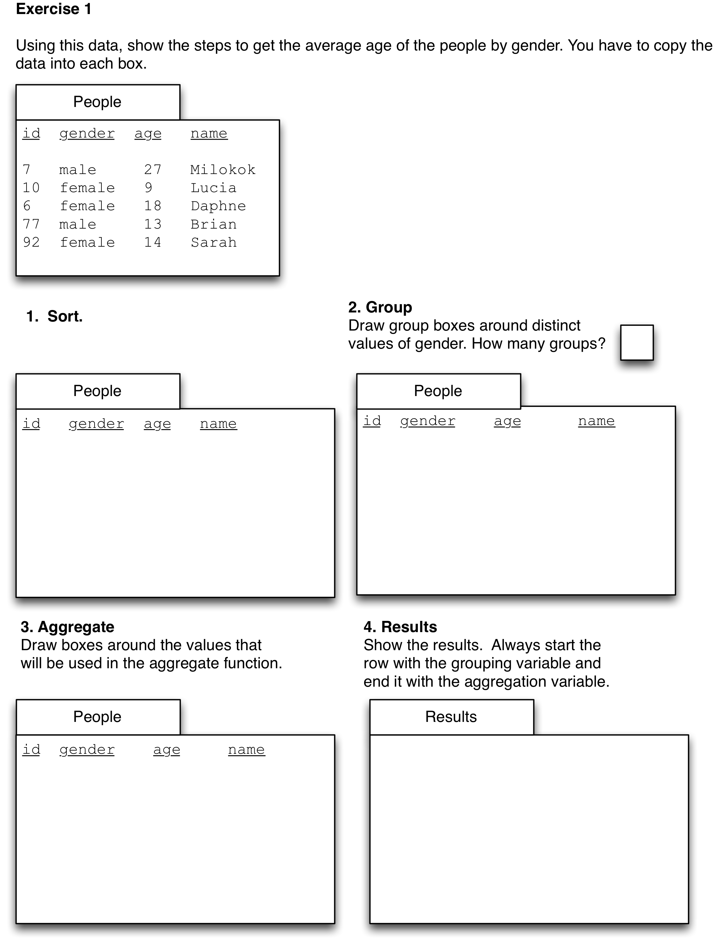
Grouping Handout
Below is a handout that we filled out with a pen in class. If you are working on this after class, you can load this into any program that lets you write text over the boxes (e.g., Preview.app, PowerPoint, Google Draw, Miro).
More than one row per group (aka windowing)
In the examples so far we have reduced our groups in only one way, by adding up values in the weight_in_grams columns. We could equally do other things that reduce to a single row per group, such as taking the average or the median instead of adding them up.
We can also do things that result in more than one row per group. This is often called “windowing” for the idea that we move down the sorted groups with a window of fixed size.
For example, we can reduce our group by sorting within them and taking only the top few rows. Here are some cars with data on Manufacturer, the year the model was produced and the miles_per_gallon on the highway. This is a longer data frame (47 rows) so I’m just showing the first and last few rows.
| manufactuer | year_produced | model | miles_per_gallon_highway | |
|---|---|---|---|---|
| 1 | Ford | 2017 | GT | 18 |
| 2 | Ferrari | 2015 | 458 Speciale | 17 |
| 3 | Ferrari | 2015 | 458 Spider | 17 |
| 4 | Ferrari | 2014 | 458 Italia | 17 |
| 5 | Ferrari | 2016 | 488 GTB | 22 |
| 6..43 | ||||
| 44 | Porsche | 2016 | Panamera | 28 |
| 45 | McLaren | 2016 | 570 | 23 |
| 46 | Rolls-Royce | 2016 | Dawn | 19 |
| 47 | Rolls-Royce | 2016 | Wraith | 21 |
We can get the top 3 most efficient cars for each year (regardless of manufacturer), sorting the table by the year produced. We can then draw a line across the table where the year value changes. We have a small group for 2014, a few more for 2015, a whole load in 2016, and a few in 2017.
| manufacturer | year_produced | model | miles_per_gallon_highway |
|---|---|---|---|
| Ferrari | 2014 | 458 Italia | 17 |
| Lamborghini | 2014 | Gallardo | 20 |
| Ferrari | 2015 | 458 Speciale | 17 |
| Ferrari | 2015 | 458 Spider | 17 |
| Ferrari | 2015 | California | 23 |
| Ferrari | 2015 | FF | 16 |
| Ferrari | 2015 | F12Berlinetta | 16 |
| Ferrari | 2015 | LaFerrari | 16 |
| Lamborghini | 2015 | Aventador | 18 |
| Lamborghini | 2015 | Huracan | 20 |
| Audi | 2015 | R8 | 20 |
| Ferrari | 2016 | 488 GTB | 22 |
| Nissan | 2016 | GT-R | 22 |
| Bentley | 2016 | Continental GT | 25 |
| Maserati | 2016 | Granturismo | 21 |
| Maserati | 2016 | Quattroporte | 23 |
| Maserati | 2016 | Ghibli | 24 |
| BMW | 2016 | 6-Series | 30 |
| BMW | 2016 | i8 | 29 |
| BMW | 2016 | M4 | 24 |
| BMW | 2016 | M5 | 22 |
| BMW | 2016 | M6 | 22 |
| Aston Martin | 2016 | Rapide S | 21 |
| Aston Martin | 2016 | Vanquish | 21 |
| Aston Martin | 2016 | Vantage | 19 |
| Chevrolet | 2016 | Corvette | 22 |
| Audi | 2016 | RS 7 | 25 |
| Audi | 2016 | S6 | 27 |
| Audi | 2016 | S7 | 27 |
| Audi | 2016 | S8 | 25 |
| Jaguar | 2016 | F-Type | 24 |
| Mercedes-Benz | 2016 | AMG GT | 22 |
| Mercedes-Benz | 2016 | SL-Class | 27 |
| Porsche | 2016 | 911 | 28 |
| Porsche | 2016 | Panamera | 28 |
| McLaren | 2016 | 570 | 23 |
| Rolls-Royce | 2016 | Dawn | 19 |
| Rolls-Royce | 2016 | Wraith | 21 |
| Ford | 2017 | GT | 18 |
| Ferrari | 2017 | GTC4Lusso | 17 |
| Acura | 2017 | NSX | 22 |
| Aston Martin | 2017 | DB11 | 21 |
| Dodge | 2017 | Viper | 19 |
| Lotus | 2017 | Evora | 24 |
| Tesla | 2017 | Model S | NA |
| Porsche | 2017 | 718 Boxster | 28 |
| Porsche | 2017 | 718 Cayman | 29 |
Then we can sort within each group, rearranging the rows to bring the more efficient cars to the top of each group.
| manufacturer | year_produced | model | miles_per_gallon_highway |
|---|---|---|---|
| Lamborghini | 2014 | Gallardo | 20 |
| Ferrari | 2014 | 458 Italia | 17 |
| Ferrari | 2015 | California | 23 |
| Lamborghini | 2015 | Huracan | 20 |
| Audi | 2015 | R8 | 20 |
| Lamborghini | 2015 | Aventador | 18 |
| Ferrari | 2015 | 458 Speciale | 17 |
| Ferrari | 2015 | 458 Spider | 17 |
| Ferrari | 2015 | FF | 16 |
| Ferrari | 2015 | F12Berlinetta | 16 |
| Ferrari | 2015 | LaFerrari | 16 |
| BMW | 2016 | 6-Series | 30 |
| BMW | 2016 | i8 | 29 |
| Porsche | 2016 | 911 | 28 |
| Porsche | 2016 | Panamera | 28 |
| Audi | 2016 | S6 | 27 |
| Audi | 2016 | S7 | 27 |
| Mercedes-Benz | 2016 | SL-Class | 27 |
| Bentley | 2016 | Continental GT | 25 |
| Audi | 2016 | RS 7 | 25 |
| Audi | 2016 | S8 | 25 |
| Maserati | 2016 | Ghibli | 24 |
| BMW | 2016 | M4 | 24 |
| Jaguar | 2016 | F-Type | 24 |
| Maserati | 2016 | Quattroporte | 23 |
| McLaren | 2016 | 570 | 23 |
| Ferrari | 2016 | 488 GTB | 22 |
| Nissan | 2016 | GT-R | 22 |
| BMW | 2016 | M5 | 22 |
| BMW | 2016 | M6 | 22 |
| Chevrolet | 2016 | Corvette | 22 |
| Mercedes-Benz | 2016 | AMG GT | 22 |
| Maserati | 2016 | Granturismo | 21 |
| Aston Martin | 2016 | Rapide S | 21 |
| Aston Martin | 2016 | Vanquish | 21 |
| Rolls-Royce | 2016 | Wraith | 21 |
| Aston Martin | 2016 | Vantage | 19 |
| Rolls-Royce | 2016 | Dawn | 19 |
| Porsche | 2017 | 718 Cayman | 29 |
| Porsche | 2017 | 718 Boxster | 28 |
| Lotus | 2017 | Evora | 24 |
| Acura | 2017 | NSX | 22 |
| Aston Martin | 2017 | DB11 | 21 |
| Dodge | 2017 | Viper | 19 |
| Ford | 2017 | GT | 18 |
| Ferrari | 2017 | GTC4Lusso | 17 |
| Tesla | 2017 | Model S | NA |
Finally we can reduce each group by taking just the top 3 rows within the group (picking at random if ties). 2014 only has 2 rows, so both of those are included.
| manufacturer | year_produced | model | miles_per_gallon_highway |
|---|---|---|---|
| Lamborghini | 2014 | Gallardo | 20 |
| Ferrari | 2014 | 458 Italia | 17 |
| Ferrari | 2015 | California | 23 |
| Lamborghini | 2015 | Huracan | 20 |
| Audi | 2015 | R8 | 20 |
| BMW | 2016 | 6-Series | 30 |
| BMW | 2016 | i8 | 29 |
| Porsche | 2016 | 911 | 28 |
| Porsche | 2017 | 718 Cayman | 29 |
| Porsche | 2017 | 718 Boxster | 28 |
| Lotus | 2017 | Evora | 24 |