15  Excel Queries

Excel is a powerful tool; you can do many of the same things we’ve been doing in SQL in Excel. I used to claim that there were things that you couldn’t do, but I was always shown to be wrong by someone!

Having said that, Excel does things differently than SQL and definitely has trouble with lots of data. That is for two reasons:

First, Excel always shows all the data, so it all has to be in the computer’s active memory (RAM), whereas SQL keeps things on disk. That can make things like scrolling through the data slow and laggy.

Second, Excel doesn’t have some of the advanced algorithms that make large joins efficient.

15.1 Excel for tabular data.

Excel arranges data in rows and columns, just like SQL. However, the columns are not like fields in SQL in that they are not “strongly typed” (meaning that you could have regular text in a column right above a date or a number) and the structure of columns and rows is not tightly enforced (you could have one row with 5 columns and the next row having only 3, or a “table” with lots of footnotes or even multiple tables per worksheet).

In fact it’s better to think of Excel in its default state as closer to a word processor (like Word) using fancy tables (which is not to say that you can’t change the defaults to enforce datatypes, just that the defaults are not like that).

Excel also doesn’t have a strong concept of a row that groups the elements together. So it’s possible to end up moving data in a field to a different row, something that sometimes happens accidentally. In a sheet that has people, their names and their ages, you might end up swapping one person’s “age” with another person, not typically something you want to do!

Excel allows multiple “Worksheets.” These are used like tabs in a browser; they can hold separate data, but can also hold user interface elements, like graphs or even laid-out text. So you can sometimes think of worksheets as like different tables in SQL, but keep in mind that while they can work like that, they don’t always.

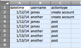
Almost all we’re going to explore in Excel relies on having data set up as tabular data, very similar to tables in SQL: columns (with headers) and rows of data, each row representing a different record (or instance of an Entity).

15.2 Sorting and Filtering

When you have an excel sheet set up with data in columns and rows, you can do sorting and filtering, just as we did in SQL.

Sorting requires selecting the data first. Be careful here as it’s possible to select only a subset of the data, leaving parts of it unsorted (if you leave off rows), or breaking up rows (if you leave off columns). I typically either select the whole sheet (clicking in the upper left hand corner of the worksheet, see the little triangle thing?) or select the columns I want to sort by clicking on the column headers and dragging across.

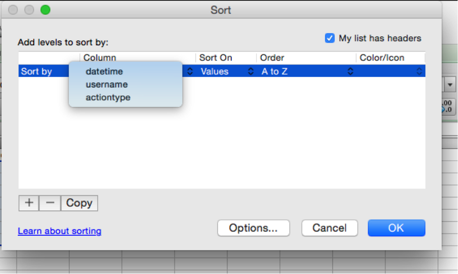
You can then choose Data -> Sort from the menus. Be sure to check “My list has headers”. The sort panel looks like this (I’ve clicked in the Column column). You can sort by multiple columns (just like ORDER BY two fields) by clicking the + symbol and adding a second sort condition.

15.3 Filtering

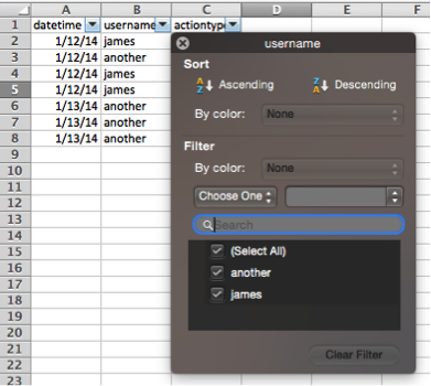
Filtering is Excel’s equivalent to conditions in SQL’s WHERE which just knock out rows like venues.name = "BMI". Filters hide rows.

There are many options for filtering, but an immediately useful one is to turn filtering on by choosing Data -> Filter from the menus. That creates a drop down on the first row (headers). Data -> Advanced Filters can copy the result of filtering to another sheet.

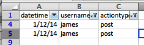
When you have a filter set the tiny icon on the table header changes and the row numbers are highlighted in blue (indicating hidden rows). Below I have two filters set (one on username, one on actiontype).

15.4 Calculations

Excel’s strength is in calculations, doing things like adding up columns of numbers or multiplying one cell by the contents of another. This reflects Excel’s accounting heritage. Using these features we can achieve things similar to both aggregate functions in SQL (COUNT, SUM and AVG) and math in the SELECT/SET clauses (SET bands.fee = bands.fee + 100)

Calculations are done via formulas which are indicated by typing text into a cell starting with the = sign. Unlike SQL Formulas refer to locations on the worksheets by using the column letters and row numbers and not using headers (or column titles). Thus A2 refers to the cell in the first column, but in the second row. We enter a formula into a cell where we want the answer to appear, for example we might have the number 7 in A1 and the number 7 in B1 and want to put the result in B3. In cell B3 we’d write: = A1 + B1

Here we are adding together 7 (A1) and 7 (B1) and putting the answer into B3. If we later change the value in A1 or B1, then the formula will recalculate, changing the result in B3.

If we want to do a calculation to create a new column for a tabular (“table-like”) sheet with rows and columns, we locate a new empty column (perhaps using insert) and then write the formula into the top cell, and copy the formula down the page. Roughly speaking this is the equivalent of:

SELECT ticket_price * tickets_sold AS total_revenue
FROM table

--or (after creating a column total_revenue)
UPDATE table
SET total_revenue = ticket_price * tickets_sold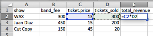

Here I’ve clicked in E2 and typed = (indicating that I want to enter a formula). Then I clicked in C2 (making it highlight blue and the click enters C2 into the formula). Then I type * (for multiply) and then click D2. When I press enter, the formula will calculate the total revenue (here tickets are all the same price).

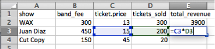
To do the same for Juan Diaz, we’ll need to have a similar, but slightly different, formula in the cell E3. Rather than having the number 2 in the formula we’ll have the number 3. Happily, Excel understands this and thinks about where the formula is being pasted from and where it is pasted to, and changes the numbers accordingly. So if you select E2, choose copy, and then paste into E3, hit return, then double-click in E3, you’ll see that the 2s in the formula changed to 3s.

There are many ways to copy a formula down a full column. One is by dragging down the + symbol that appears when you click a cell and hover over its bottom right corner (the mouse cursor doesn’t show up in this screen shot, but it will appear right on top of the blue square):

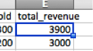
If you then click and drag down the column, Excel will “fill down” and copy the formula, again adjusting the row numbers so that each copy of the formula refers to the right row. Another way to do this is to double-click the little handle that you pulled down; if the sheet is organized like a table, then this will fill the contents of that cell down the column. Handy!

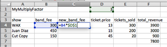
Note: if you don’t want Excel to change the row or column automatically (e.g., you want to multiply a whole column by the value of a single cell (not a cell changing for each row), then you put a $ in front of the element you don’t want to change. E.g.: instead of D1 we have $D$1, then when we copy down to C5 the formula will still reference D1 (instead of changing to D2). You can “fix” parts of the formula (rows or columns), so you can have $D1 or D$1 depending on whether you want to let rows or columns vary.

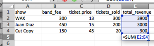
You can produce totals of columns, like using SUM() in SQL. In fact it’s the same function name:

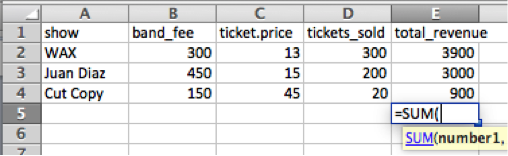
Here I’ve clicked in E5 and typed =SUM(. To indicate what cells you’d like to add up, you have to enter a range, which is done as the name of the starting cell, then a colon, then the name of the ending cell. You can get this by clicking and dragging over the cells (then typing close parens).

15.5 Something like a join

Excel doesn’t have real joins, but you can do something very similar. Note, though, that this can be very slow with lots of data; it’s not something I’d choose to do often, but it can be handy, especially when working with collaborators that function in Excel only.

Here we have some data from a web log, showing a datetime, the name of a user and the sort of action that the user took, here either join for when they joined the site (nothing to do with a database join!), or post for when they posted something on the site. We might want to add some data, indicating that particular users are acting as managers or volunteer moderators.

datetime	user_name	action_type
2011-06-03	James Howison	join
2011-06-04	James Howison	post
2011-06-02	Lord Vader	join
…	…	…

You want to add a column saying whether the user in that row is a “manager” or “volunteer”. Of course you could do this manually, but with many, many rows of data that’s not a great idea. You can use another Excel worksheet to create a table with the related data about the user:

|user_name|user_type| |James Howison|manager| |Lord Vader|volunteer| |…|…|

We want to join on user_name and bring the user_type attribute to the joined table.

datetime	user_name	action_type	user_type
2011-06-03	James Howison	join	manager
2011-06-04	James Howison	post	manager
2011-06-02	Lord Vader	join	volunteer
…	…	…	…

This is a database join, even though we aren’t using primary and foreign keys (ids). In SQL you could do it like this (recall that a join means that all rows are mixed together in a big cross-product and then those that don’t meet the condition are eliminated, that logic works just the same when working with text columns as it does working with id columns.)

SELECT *
FROM log
 JOIN roles ON log.user_name = roles.user_name

However we don’t have a database join operation available (In the Microsoft world JOIN is only available for their Access or SQLServer products). So we can use either VLOOKUP or INDEX MATCH (which are Excel functions). INDEX MATCH is much more flexible, so that’s what we’ll learn.

15.5.1 Data for excel join

Download this excel file which combines the two csv files, one per tab. If you want to practice importing csv into your Excel file (every version works slightly differently) you can get the original csv files here:

1. log_data.csv - shows events by users
2. user_types.csv - gives a user type label for each user

If you import your own csv files, but exclude the .csv from the tab names you’ll have to changed the formulas below to match what you call the sheets. You’ll know this has happened if you get a pop-up asking you to find user_types.csv.

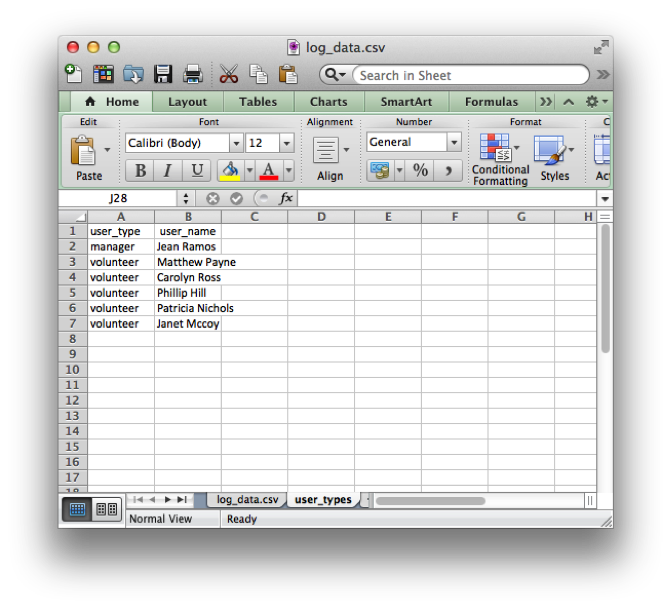
You then need to switch back to the log_data.csv sheet and put together the INDEX MATCH formula. This will look at column B on the user_types.csv worksheet (the user_name), then look at column B on the other worksheet, if they match it will copy the content of the user_type column over to column D in the first worksheet.

Because we’re copying into column D that is where we put the formula.

=INDEX(user_types.csv!$A$2:$A$7,MATCH(log_data.csv!$B2,user_types.csv!$B$2:$B$7,0))

The formula is a bit complicated, but it is well explained here How to use INDEX MATCH.

15.5.2 Filling NAs

For the rows where there are no matches, the formula leaves NAs (like a NULL value in SQL), in Excel NA stands for “Not Available”. So if we have a “everyone else” category, such as “user” (not a “manager” nor a “volunteer”), then we can convert all the NAs to the “user” category.

So we need to alter the formula a bit, asking that if the formula returns NA then use the value “user”. This looks complicated and it has three parts: 1) the test, 2) the value if the test was true, and 3) the value if the test was false.

The test is our original formula:

=INDEX(user_types.csv!$A$2:$A$7,MATCH(log_data.csv!$B2,user_types.csv!$B$2:$B$7,0))

And it gets surround by two other formulas an IF and an ISNA.

If the original formula returns “NA” then the value for true is “user” and if the original forumla didn’t return an “NA” (ie false) then the value should be whatever our original formula would have returned, but we express that by just repeating our formula:

Together this looks like:

=IF(
   ISNA(
       INDEX(user_types.csv!$A$2:$A$7,MATCH(log_data.csv!$B2,user_types.csv!$B$2:$B$7,0))
   ),
   "user",
   INDEX(user_types.csv!$A$2:$A$7,MATCH(log_data.csv!$B2,user_types.csv!$B$2:$B$7,0))
)

Ugly, but hey, you are doing JOIN in Excel!