Tidyverse Extras
Some additional R tidyverse aspects covered here to maintain the flow of techniques on the main page.
Accessing Rstudio
For this course we have access to Rstudio via EduPod, a service provided by UTexas. You can log in using your lower-case EID/password at https://edupod.cns.utexas.edu/
This provides a separate workspace for each student and gives access to Rstudio. You will be able to upload files into the workspace and your files will persist between logins.
For support with logging in or configuration issues you should email mailto:rctf-support@utexas.edu
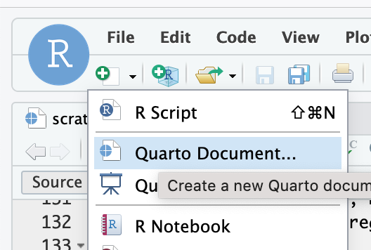
In general I recommend that you work with Quarto Documents producing HTML output. You can create a new document using the File menu in Rstudio.
Quarto gives us a Notebook environment, which is a mix of Code cells and textual content. We execute code within code cells (which have grey backgrounds).
To get started you should right-click and save this file to your laptop.
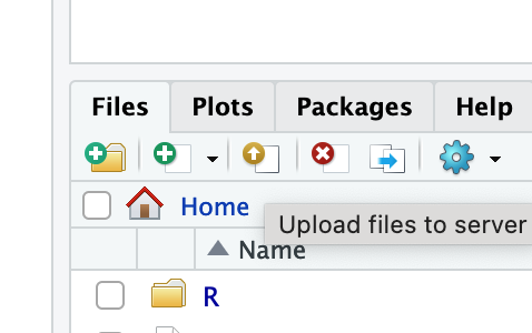
You can then upload it using the Files part of the Rstudio interface, using the little gold colored upload arrow.
Datatypes
When we load data from files we get either numbers or text. For example, a csv file might look like:
customer_name,customer_age
Harry,9
Dumbledore,90
But inside our frameworks we can have lots of other kinds of data. Dates and times are a good example. If we know that a column is about time we can do quite a few useful things with it:
- Change how the datetime is formatted (e.g., convert from YYYY-MM-DD to DD-MM-YYYY)
- Add units of time (e.g., add 35 days to 12 Feb 2024)
- Nicely format graph axes and labels
Some columns can include what we call a categorical variable. A good example is Low, Medium, and High. This is categorical because it is a list of category labels. Categorial variables have a limited number of values that they can take (here that number is 3). Saying that a column is categorical lets us do useful things such as specifying an order that these values should be shown in a graph (ie we would usually want to show “Low” then “Medium” then “High”.)
Here is a summary of datatypes in the R tidyverse. The left column is a general name that we can use loosely across all of our frameworks. The second column shows what R calls this type of data, and the third column shows how we would write this sort of data in R code. Finally we show the function that we would use (note that sometimes these have a dot, like as.character and sometimes they have an underscore, like as_datetime). When tidyverse has a package that particularly helps I include it below.
| descriptor | example | r_name | abbrev | conversion_function |
|---|---|---|---|---|
| General text | "Austin in Texas" | character | chr | as.character(col_name) |
| Numbers | 67 or 67.4332 | numeric or double | dbl | as.numeric(col_name) |
| True/False | TRUE or T or 1, | logical | lgl | as.logical(col_name) |
| Dates and times | "2014-09-34 12:34:22" | datetime | POSIXct | as_datetime(col_name) |
| Categorical Variables | c("Low", "High") | factor | fctr | fct(col_name, levels = c("Low", "High")) |
Here is how we would convert a column to a particular datatype (using the conversion function inside mutate).
products |>
  mutate(price_in_dollars = as.numeric(price_in_dollars))
Dealing with dates and times
Data with dates and times comes in lots of different forms. You might get 10-03-2024 or October 3, 2024 or 3rd of October 2024. You might even get time looking like 1726290000 (which is the number of seconds since start of 1970, nifty!) Happily our frameworks can help us interpret these; while the range of formats is high it isn’t unlimited!
We usually have two options. We can provide a template string telling the framework what to expect (and then getting an error if rows do not match) or we can let the framework guess (trying as many options as it can). We can also give a list of possible options.
tribble(
  ~report_date, ~report_text,
  "2004-08-23", "Wow, speedy cigar shaped object",
  "3 October, 1992", "Saw a round plate zoom past",
  "04-05-2010", "Crikey, saw a beaut of a ufo"
)  |>
  mutate(report_date_norm = parse_date_time(report_date, orders = c("ymd", "dmy", "dby")))
The parse_date_time function comes from lubridate which is part of the tidyverse set of packages. It uses these little strings that it calls “orders” such as “ymd” (year month day) and “dby” (day month_as_word year). They are documented on the lubridate documentation, and include little codes for time as well (e.g., ymd HMS).
Dates from Excel
Excel has a difficult habit of storing a number in a cell, but displaying that number as a date. So when you load an Excel file, you may see dates represented as numbers like 42370.
That is … wait for it … the number of days since December 31, 1899 (it’s a bit more complicated). parse_date_time does not directly handle these numbers. read_excel importing function does a great job, but doesn’t always convert columns with Dates or Datetimes correctly (especially when the column contains mixed data, such as truncated dates). See more here in an Issue filed at the read_excel github
Thankfully janitor::convert_to_datetime function can handle these specific Excel dates.
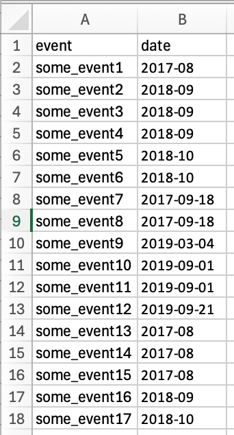
Here is an example Excel file, which contains mixed dates in one column. It looks like this opened in Excel:
If we load that into R, using read_excel we can see how the date column comes in.
library(readxl)
mixed_dates <- read_excel("assets/mixed_date_column.xlsx")

mixed_dates
So the column has been understood as chr but the full Excel dates are now showing with their internal Excel representation of numbers like 43528.
We can handle this using a combination of janitor::convert_to_datetime for the Excel dates, then falling back to lubridate::parse_date_time for the truncated dates.
mixed_dates |>
  mutate(fixed_date = janitor::convert_to_datetime(date,
                                                   character_fun = lubridate::parse_date_time,
                                                   orders = "ymd", truncated = 1, tz = "UTC"))
It seems like it is only mixed dates; the Excel file above has another tab with only full dates and that seems to load fine, whether Excel knows these are date formatted cells or not.
library(readxl)
read_excel("assets/mixed_date_column.xlsx", sheet = "full_dates")
It isn’t just truncated dates that cause the issue, the third tab has all full dates but one row has “???” perhaps someone manually entered that to show that they didn’t know the dates.
library(readxl)
read_excel("assets/mixed_date_column.xlsx", sheet = "mixed_dates_and_text")
To handle that you can use a case_when before the convert_to_datetime. Or you can use the string_conversion_failure = "warning" parameter which will convert those it can, but give an NA for those it can’t.
read_excel("assets/mixed_date_column.xlsx", sheet = "mixed_dates_and_text") |>
  mutate(fixed_date = janitor::convert_to_datetime(date, string_conversion_failure = "warning"))
Warning: There were 2 warnings in `mutate()`.
The first warning was:
ℹ In argument: `fixed_date = janitor::convert_to_datetime(date,
string_conversion_failure = "warning")`.
Caused by warning:
! All formats failed to parse. No formats found.
ℹ Run `dplyr::last_dplyr_warnings()` to see the 1 remaining warning.More on Factors
Factors in R are very useful and we will work with them using the forcats package that is part of tidyverse. Factors hold categorical variables, with the valid values allowed called levels of the factor. So we would say,
The
country_wealthcolumn is a factor with the levels Low, Medium, or High.
We can convert a column of text into factors using fct(col_name). If we don’t specify levels then forcats turns this into a factor with levels set to the order each is first seen. For example, if we had these data coming in from a csv file, the rainfall_label column would arrive as just character. Looking at it we can see that it ought to be a factor.
We can convert it to a factor using fct in mutate
state_rainfalls |>
  mutate(rainfall_facter = fct(rainfall_label))
Now we see that the column datatype (shown in light grey under the column title) has changed from <chr> to <fctr>.
We can see a little more using the count function for our factor column. This shows us a list of the levels in order and a count of the number of times it shows up.
state_rainfalls |>
  mutate(rainfall_facter = fct(rainfall_label)) |>
  count(rainfall_facter)
So fct created a factor, but ordered the levels by the order it first saw them (as it moved down the datatable). We can override that by specifying the levels we want, in the order we want.
state_rainfalls |>
  mutate(rainfall_facter = fct(rainfall_label, levels = c("Low", "Medium", "High"))) |>
  count(rainfall_facter)
This is particularly handy for changing the order when making a figure:
state_rainfalls |>
  mutate(rainfall_facter = fct(rainfall_label, levels = c("Low", "Medium", "High"))) |>
  ggplot(aes(x = rainfall_facter)) +
  geom_bar()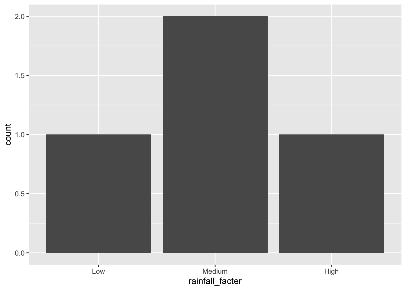
If we change the order of the factor levels, then the order of the categories on the x axis are changed.
state_rainfalls |>
  mutate(rainfall_facter = fct(rainfall_label, levels = c("Medium", "Low", "High"))) |>
  ggplot(aes(x = rainfall_facter)) +
  geom_bar()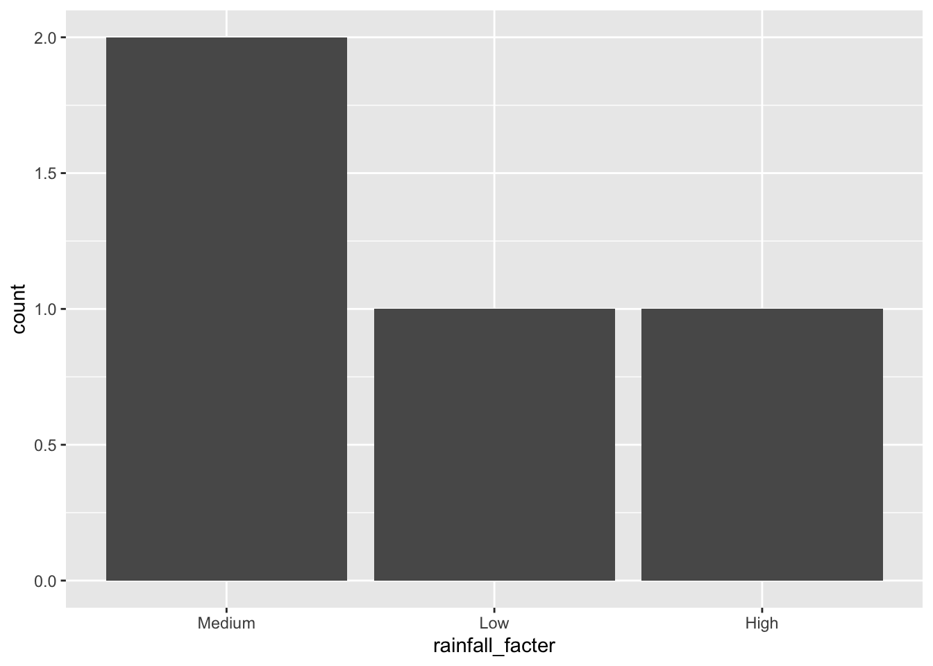
Factors can be really helpful to validate data as well. For example, if we are only expecting values for “Low” and “High” then fct will throw an error.
state_rainfalls |>
   mutate(rainfall_facter = fct(rainfall_label, levels = c("Low", "High")))
Error in `mutate()`:
ℹ In argument: `rainfall_facter = fct(rainfall_label, levels = c("Low",
"High"))`.
Caused by error in `fct()`:
! All values of `x` must appear in `levels` or `na`
ℹ Missing level: "Medium"case_when for factor from numerical
Often it is useful to convert a numerical value into categories for analysis. We can do this manually using case_when. Here I’m using data from the US “General Social Survey” which has a row per (anonymized) respondent, and has data on hours of television watched.
| id | marital | tvhours | |
|---|---|---|---|
| 1 | 1 | Never married | 12 |
| 2 | 3 | Widowed | 2 |
| 3 | 4 | Never married | 4 |
| 4 | 5 | Divorced | 1 |
| 5 | 7 | Never married | 3 |
| 6..1828 | |||
| 1829 | 2817 | Divorced | 2 |
We can create categories for the tvhours variable, using case_when inside a mutate to create a new column. We use two calls to mutate here, first creating a column that contains characters, then converting that to a factor with levels.
tv_gss |>
  mutate(tv_category = case_when(
                        tvhours <= 3 ~ "Low",
                        tvhours <= 6 ~ "Medium",  # between 3 and 6 because checked after first option
                        tvhours <= 9 ~ "High",
                        10 < tvhours  ~ "Extra High"),
         tv_category = fct(tv_category, levels = c("Low", "Medium", "High", "Extra High")))
Working with zip codes
Zip codes look like numbers … but what the ones that start with zero? Up in Maine. To a computer there is no number 08876 because numbers always drop leading zeros. Then it just becomes 8876 …
Zip codes also aren’t numbers because we don’t do math stuff with them. We can add them together, we can’t multiply them. We also can’t use them like a number when making figures (should 78723 be higher than 78701??)
So we should treat ZIP codes as factors, categorical variables.
tribble(
  ~full_address,
  "1616 Guadalupe, Austin, TX, 78701",
  "106 South First Stree, Austin TX, 78705",
  "20 Somewhere St, Maine, 08876"
) |>
  separate_wider_regex(full_address,
    patterns = c(address_remain = ".*?",     # anything until
                 chr_zip            = "\\d{5}$") # five digits at end
  ) |>
  mutate(dbl_zip = as.numeric(chr_zip),
         fct_zip = fct(chr_zip))
Working with missing values: NA
R uses a special value, called “an NA”, to represent missing values.
For example, in the data set about cars we have a miles_per_gallon_highway column. But one type of car has an NA in that spot. The one Tesla in the dataset just doesn’t have a value for miles_per_gallon_highway … which makes sense since it doesn’t use gallons of gas.
my_cars <- gtcars %>%
  select(manufacturer = mfr, year_produced = year, model, miles_per_gallon_highway = mpg_h) %>%
  filter(manufacturer %in% c("Ford", "Audi", "Tesla"))

my_cars
When we have NA values we have to figure out what we can interpret from them. For example how should the Tesla model contribute to calculating the mpg of this group of cars? R, with its statistical heritage, is aware of these sort of issues. The mean function (that gets the average of a group of numbers) just won’t give you an answer. Even a single NA is enough to make the mean return NA!
my_cars %>%
  summarize(avg_mpg = mean(miles_per_gallon_highway))
Often we can’t interpret the data with NA present, and we have no way of interpolating/estimating the missing data, so we drop the rows. This is a kind of filter or excluding rows. But NA values can be tricky to use in boolean logic and in the way R represents different datatypes. So R tidyverse provides drop_na
my_cars %>%
  drop_na(miles_per_gallon_highway) %>%
  summarize(avg_mpg = mean(miles_per_gallon_highway))
Missing or empty?
NA values are curious. They can sometimes mean that the data is not possible, but more often they mean that it is just missing … perhaps not collected or unknown, or the data was out of a sensible range.
NA values are also different from empty values. For example, imagine we are tagging photos. Each photo starts out with no tags, and we look at every photo, but only tag those that we like with “favorite” or “beautiful” (or maybe both). We could then say that the other photos have no tags, or we might say that they have an empty tag list. We have explicitly considered tagging the photo, and decided not to … and no tags is a type of data that we can interpret (perhaps marking the photos as boring or deleting them). Quite different than if we just haven’t looked at the photo yet!
When we load data from a file like a CSV, though, missing data might be represented in different ways; it even might be different in different columns! CSV doesn’t have a special NA value … it is “just text” so we may have to figure it out after we load the data.
photos_with_tags <- tribble(
  ~path, ~tags,
  "photo-1111.jpg", "beautiful",
  "photo-2222.jpg", "beautiful",
  "photo-3333.jpg", "beautiful, favorite",
  "photo-4444.jpg", NA,
)

photos_with_tags
Notice here that R shows us an NA value for the tag_list on for photo4444.jpg inside the cell is just empty … by default read_csv interprets an empty string as being NA.
But we know that all these photos have been looked at, so we can interpret that empty string as “looked at but no tags assigned”. We can replace the NA with an empty string … but the data will be easier to understand if we also add a column or two.
photos_with_status <- photos_with_tags |>
  mutate(tag_status = "tagging complete") |> # Mark every row as having been considered for tags
  mutate(tag_list = replace_na(tags, ""))

photos_with_status
Special values (like -1 or 999): na_if
Sometimes incoming datasets have used special values inside a field to indicate some special situation, often missing data. Some common ones are -1 or 999, but these can take many forms. Sometimes we can ask them people that worked with the data, but often we just have to inspect what is there and decide what is meant.
bird_observation <- tribble(
  ~bird_species, ~num_observed,
  "crows", 234,
  "grackles", 43,
  "turkeys", -1
)

bird_observation |>
  gt() |>
gt_theme_guardian() | bird_species | num_observed |
|---|---|
| crows | 234 |
| grackles | 43 |
| turkeys | -1 |
na_if can be used in these circumstances, if we decide that the special value means “unknown”. This is the reverse of replace_na ()
bird_observation %>%
  mutate(num_observed = na_if(num_observed, -1))