11 Introduction to SELECT queries
In this class we’re going to cover the basics of SQL’s SELECT query. SELECT works by applying filters to the table, filtering out data you don’t want to see, and returning data that you do want to see. The returned data ends up in a new table which has just the columns and rows that you asked for.
In the first class we used cards to build up our table representation. When we use a query it is as though we have a box that hides everything but a single row, then we ask the query about the single row and it is always one of true or false. If the answer was true then we copy the data from that row into a table called results. This is precisely how a SELECT query works.
The steps in a SELECT query are:
- Identify the table you are asking for data from
- Specify the conditions you want to ask for each row
- Specify the columns you want to copy from those rows
These correspond to different parts of the query. Somewhat oddly, though, the parts aren’t in the order above.
SELECT [columns]
FROM   [tables]
WHERE  [conditions about rows]
I wait until the end to specify the columns I want to see, so I start my queries with SELECT * where the star means “all columns”.
We will build our queries up step by step inside a notebook. This is a little laborious but as our queries become more complex (especially as we work with more than one table) you’ll find that this habit serves you very well.
The WHERE clause: picking rows using conditions
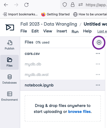
To run these queries we need to have a file called cars.csv available. You should:
- Download the cars.csv file and save it to your laptop.
- Upload the file into your DataCamp workspace.
Each row in the database represents a single car model and there are 234 car models in the database (I reduced the full set by only including cars produced in 1999 and 2008). On each row we have data about one car, such as the year it was produced (cars.year), the manufacturer (cars.manufacturer) (e.g., audi, ford), the model (e.g., a4, focus). Using a select query we can narrow the database to find cars that match our query.
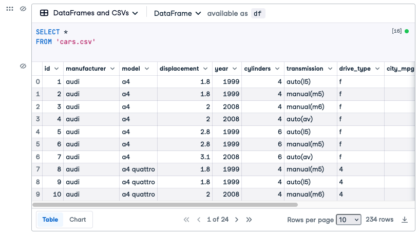
Let’s say we are interested in cars that have four cylinders. The cars.cylinders column has that information. We start by confirming that we are addressing the right table by executing this query:
SELECT *
FROM 'cars.csv'
This asks for all the data in the table and will return 234 rows and all the columns. There is no WHERE clause, which means that there are no conditions on the rows and that is why all of them are returned. When you run it the results will look like this:
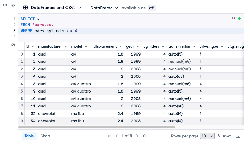
If we want to add some conditions we can add a WHERE clause:
SELECT *
FROM 'cars.csv'
WHERE cars.cylinders = 4
Now we will only see rows where the condition in the WHERE clause is true. It’s just the same as using the paper template: the computer looks at one row at a time and checks the number in the cylinders column. If that number is a 4 then the whole row is copied into the results. If you run that query, by copying the query above and pasting it (go ahead and try it now) you’ll see that the results have 81 rows (although the 81 rows are broken up into multiple screens). Every one of the rows has a 4 in the cylinders column.
We can add more conditions to our WHERE clause to reduce the number of rows shown even more. For example, let’s say that from those 4 cylinder cars we want to find older cars, produced earlier than the year 2000. We can do that by adding a condition to the WHERE clause:
SELECT *
FROM 'cars.csv'
WHERE cars.cylinders = 4
  AND cars.year < 2000
Two things to notice here. The AND and the < (less than) sign. First we use the word AND between our two conditions. I place it under the WHERE, indenting it by two spaces to show that it is still part of the WHERE clause and causing the conditions to line up down the page. You could equally see this with the WHERE clause written on one line WHERE cars.cylinders = 4 AND cars.year < 2000 But I prefer to have one condition per line, to keep things visually neat.
The < (less than) sign will allow more than one value in the row, as long as it is below 2000. (It would exclude rows with year = 2000, since we used < (less than) and not <= which is less than or equal to.). If we run this query we see our results reduced from 81 to 45 cars.
Conditions with different data types
Our columns in SQL have datatypes associated with them (text, numbers, datetimes). The datatype has some impact on how we write our conditions. When we are querying number columns (INT, DECIMAL) we don’t use quotes around the data we supply. See how there are no quotes around 4 and 2000 in this query:
SELECT *
FROM 'cars.csv'
WHERE cars.cylinders = 4
  AND cars.year < 2000
But if we’re writing a condition on a non-number field we need to use quotes around the bit we supply. e.g.,
SELECT *
FROM 'cars.csv'
WHERE cars.manufacturer = 'audi'
We also need quotes around date fields cars.production_date = '2008-06-06'. You must use single quotes, for the particular database we are using.
Boolean Algebra (resolving AND and OR)
The WHERE clause in the query above is asking three questions of each row, each of which resolves to TRUE or FALSE. Three? I only see two! (you say). Well here are the three:
- Is the value for
cylinderson this row equal to 4? –> TRUE or FALSE - Is the value for
yearon this row less than 2000 –> TRUE or FALSE - Was the answer to questions 1 and 2 both TRUE? –> TRUE or FALSE.
For 4 cylinder and year of 2008
cars.cylinders = 4 AND cars.year < 2000
     TRUE          AND      FALSE
                  FALSE
For 4 cylinder and year of 1999
cars.cylinders = 4 AND cars.year < 2000
     TRUE          AND      TRUE
                  TRUE
This is called Boolean Algebra, which you may have heard of. It’s a way of reducing a combination of conditions down to a single TRUE or FALSE value. That’s what happens here, in the first round we reduce each condition to a TRUE or FALSE (e.g., TRUE AND FALSE on the second lines above) and in the second round we reduce again (TRUE AND FALSE –> FALSE (because both were not TRUE)). These end up looking like an upside down pyramid.
This ends up more intuitive than you might be feeling at the moment. The key thing is that when you join conditions with AND all of the conditions must be true for the row to be in the results.
In addition to AND we can also join conditions with OR. When we do that we are saying that we want the row if any of the conditions are TRUE. OR ends up used much less than AND in sql.
Let’s say that we wanted all the cars but only if they were made by Audi or Ford. We would write:
SELECT *
FROM 'cars.csv'
WHERE cars.manufacturer = 'audi'
   OR cars.manufacturer = 'ford'
That works fine and we get 43 results. Things can get tricky with OR if you go beyond two conditions, mixing AND and OR. Consider these three queries:
SELECT *
FROM 'cars.csv'
WHERE cars.year = 2008
  AND cars.manufacturer = 'audi'
which returns 9 rows. And this:
SELECT *
FROM 'cars.csv'
WHERE cars.year = 2008
  AND cars.manufacturer = 'ford'
which returns 10 rows. So we know that if we combine the 2008 Ford cars and 2008’ Audi cars we should get 19 rows. Yet:
SELECT *
FROM 'cars.csv'
WHERE cars.year = 2008
  AND cars.manufacturer = 'ford'
   OR cars.manufacturer = 'audi'
gives us 28 results. So we have 9 extra results. Where are they coming from? See this screenshot:
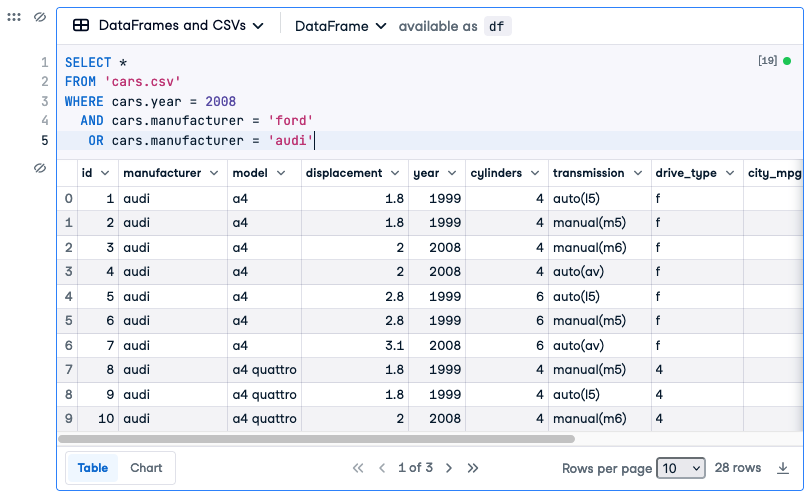
Look closely at the first row; it shows a value of 1999 for year. Why is it in the results (since 1999 most definitely is not equal to 2008).
The reason is to do with how the boolean algebra resolves. Remember that each condition is resolved first. In the figures below each clause resolves to the value written below it. So for that row (“Audi” and 1999) we would get:
cars.year = 2008 AND cars.manufacturer = 'ford' OR cars.manufacturer = 'audi'
       FALSE     AND              FALSE         OR          TRUE
The cars.year = 2008 resolves to the FALSE written under it and so on. But when we come to resolve the AND and ORs in boolean algebra the AND is resolved before the OR and thus we get:
FALSE AND FALSE OR TRUE
     FALSE      OR TRUE
               TRUE
The FALSE AND FALSE on the first line is resolved first and become a FALSE, leaving us with FALSE OR TRUE which resolves to TRUE and thus the 1999 Audi is included in the results.
What our query actually asked for was “Find me all the Fords built in 2008, and all the Audis (regardless of the year)” so as soon as a row was TRUE for the right-hand side of the OR it was included.
You can get around this by changing the order of things using parenthesis (). So we could change the order that things are resolved with:
SELECT *
FROM 'cars.csv'
WHERE cars.year = 2008
  AND (cars.manufacturer = 'ford' OR cars.manufacturer = 'audi')
Which would require every row to have 2008 for its year and either Ford or Audi for its manufacturer. This is very useful. I encourage you to always use parens whenever you use any ORs in your queries. It just makes things much easier.
Use IN rather than OR (most of the time)
Even easier still is using the IN keyword, which you should do whenever you have a list of alternatives for a value:
SELECT *
FROM 'cars.csv'
WHERE cars.year = 2008
  AND cars.manufacturer IN ('ford', 'audi')
which returns the 19 rows that we expected.
Other operators
Above we’ve used two operators inside the parts of our WHERE: the equals sing =, the < sign, and the IN keyword. There are many other operators, such as >, >= and so on.
There are also operators that do the reverse of these. Thus I can also say “not equal”: != or <> or the reverse of IN which is NOT IN (values from the list that follows will be excluded from the results.).
Finally there are a set of useful operators, such as BETWEEN operator that simplifies range queries. eg. cars.cylinders BETWEEN 4 AND 6 or, if we were using dates: cars.production_date BETWEEN '2008-03-01' AND '2009-06-05'
The SELECT clause: specifying columns
The first clause in the query specifies the columns that you want to see in the results. Compared to understanding boolean algebra this bit is easy. You supply a comma-separated list of column headings after the SELECT (instead of the *). So if we only wanted the manufacturer and model we could write:
SELECT cars.manufacturer, cars.model
FROM 'cars.csv'
WHERE cars.year = 2008
You can think of querying like this as a process of hiding, knocking out, or covering up parts of the original table that you don’t want. So if WHERE knocks rows out from your results, SELECT knocks out columns from your results.
Down the track we’ll learn other things we can do in the SELECT part of the query (such as combining columns or doing math between columns).
Doing math in the SELECT clause
The SELECT part of the query let’s us specify the columns that we want, but we can also do some basic math to derive new values.
For example, imagine a table with data about a retail store, a row for each month and a column for expenses and a column for sales.
stores(id, month, expenses, sales)If sales is our incoming money and expenses is our outgoing money, it would be useful to find the difference between them. We can do that in SQL using the minus sign -:
SELECT stores.sales, stores.expenses, stores.sales - stores.expenses
FROM stores
This math works on each row, subtracting the value for expenses in that row from the value in sales from that row. We use the values in the two columns to create a third column in the results.
Similarly you can add values using +, multiply values together using the * sign, and divide using the / slash character.
ORDER BY and LIMIT: Sorting results and getting top x rows
The three clauses above leave you with a results table, showing only the rows and columns that match your query. Now we’ll learn two things we can do with these results: sorting and limiting.
Let’s say that we wanted to find the more fuel efficient 4 cylinder cars for city driving. First we’d get all the 4 cylinder cars:
SELECT *
FROM 'cars.csv'
WHERE cars.cylinders = 4
Now we want to re-order the results table according to city_mpg (miles per gallon). Note that we’re reordering the results table, and not changing the original data in the database at all.
SELECT *
FROM 'cars.csv'
WHERE cars.cylinders = 4
ORDER BY city_mpg DESC
We add an ORDER BY clause saying that the rows should be ordered by the values in the city_mpg column for that row. Finally we say that we want those with the highest values first, thus our sorting order is descending which is abbreviated to DESC. The opposite is ascending, showing the smallest values at the top, shown with ASC. If you don’t put either then the results are sorted in Ascending order, but honestly it’s just clearest to always include either DESC or ASC.
Here are the results (selecting just manufacturer, model, fuel type (diesel/gas) and city_mpg):
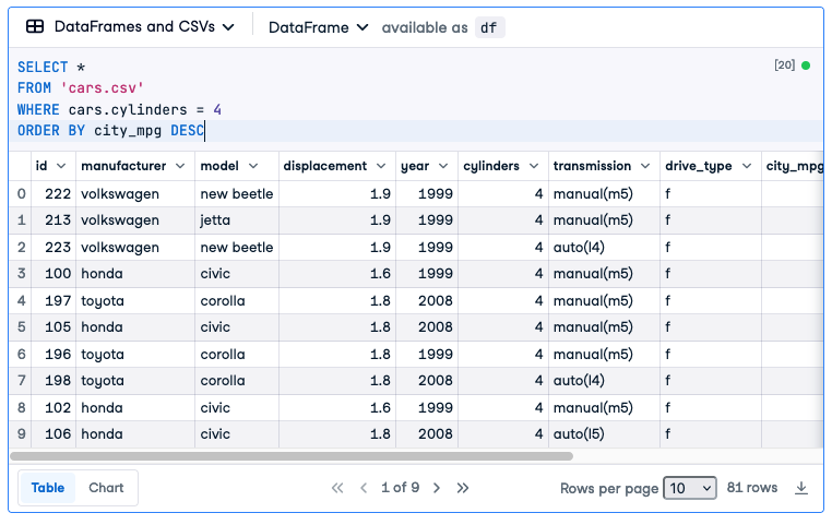
We can see that the top three are made by Volkswagen, then a Toyota Corolla and a Honda Civic and so on right through the 81 rows that return.
After we’ve sorted we often want to see just the very top result. So rather than finding the more fuel efficient cars, we find the most fuel efficient car. This is done with LIMIT 1 which means only return the first row (after sorting).
SELECT *
FROM 'cars.csv'
WHERE cars.cylinders = 4
ORDER BY city_mpg DESC
LIMIT 1
I always put LIMIT on its own line, but you will frequently see it on the end of the ORDER BY line as well. I use its own line because its clearer. You could also get the top 5 using LIMIT 5:
SELECT *
FROM 'cars.csv'
WHERE cars.cylinders = 4
ORDER BY city_mpg DESC
LIMIT 5
Summary
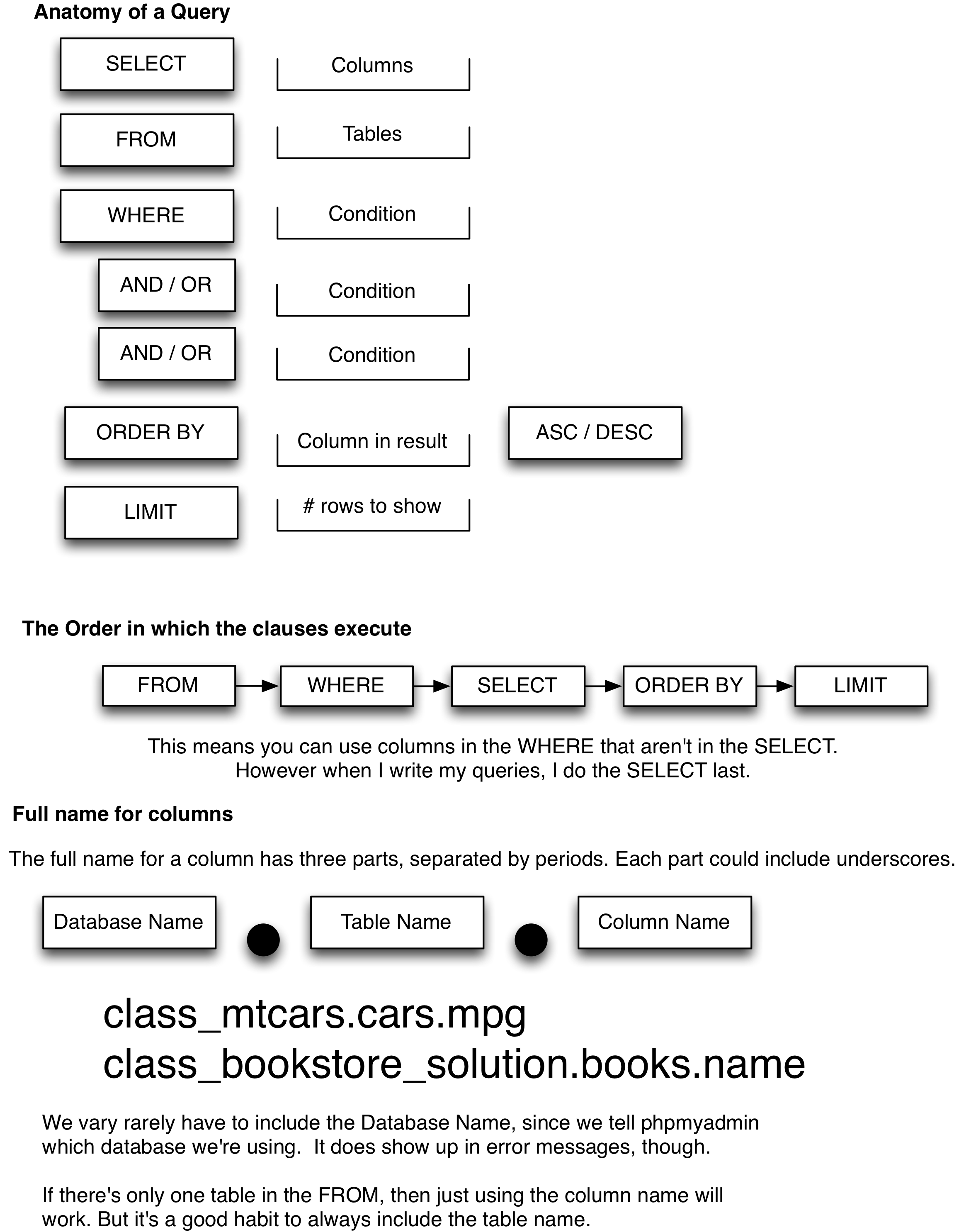
The SELECT query allows you to select data out of the table in your database. It copies rows that match the conditions in the WHERE clause (using boolean algebra) and generates a results table. You can then sort and limit the results table. The figure below shows the parts of the basic select query:
Finally as usual w3cSchool has a useful SQL tutorial. It doesn’t go in exactly the same order as we are, but it’s pretty close. Here are their materials on SQL SELECT
Exercises
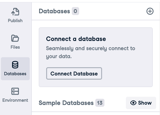
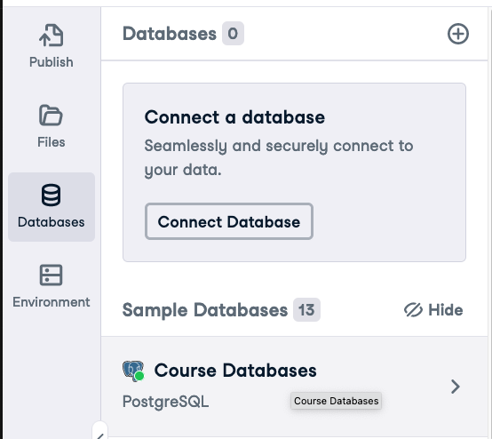
On DataCamp connect to the sample database “course_database” using the “Databases” tab on the left.
Work on these queries:
Which country has the largest surface area?
Which country became independent the last?
Which countries in Africa or Asia became independent prior to 1919?