12 Joining tables in SQL
On our first day of class we made two databases, one was a string database and one was the relational tables. One of the differences is that the string database was “all joined up” and, by following the strings, we could move across the relationships in the database.
With relational tables, though, we replaced the strings with primary keys and foreign keys. In the process we split the database up across tables. In SQL we stitch things together using “joins”. The joins we’ll learn today use the primary/foreign keys to enable us to follow the relationships across different tables. (We can also join across columns that are not primary/foreign keys, a topic we’ll return to in a class or two).
In the homework you explored one way to move between tables, by copying ids from query to query:
-- 2.4 When did Domhog Kiwter purchase his tickets?
-- Takes two steps.

SELECT people.id
FROM people
WHERE people.name = "Domhog Kiwter '

-- Intermediate Result: 71

SELECT purchases.date
FROM purchases
WHERE purchases.person_id = 71

-- Final Result: 2011-04-28 00:05:06
Joins enable us to avoid intermediate results and to follow all the relationships in the table at once, rather than just a single one.
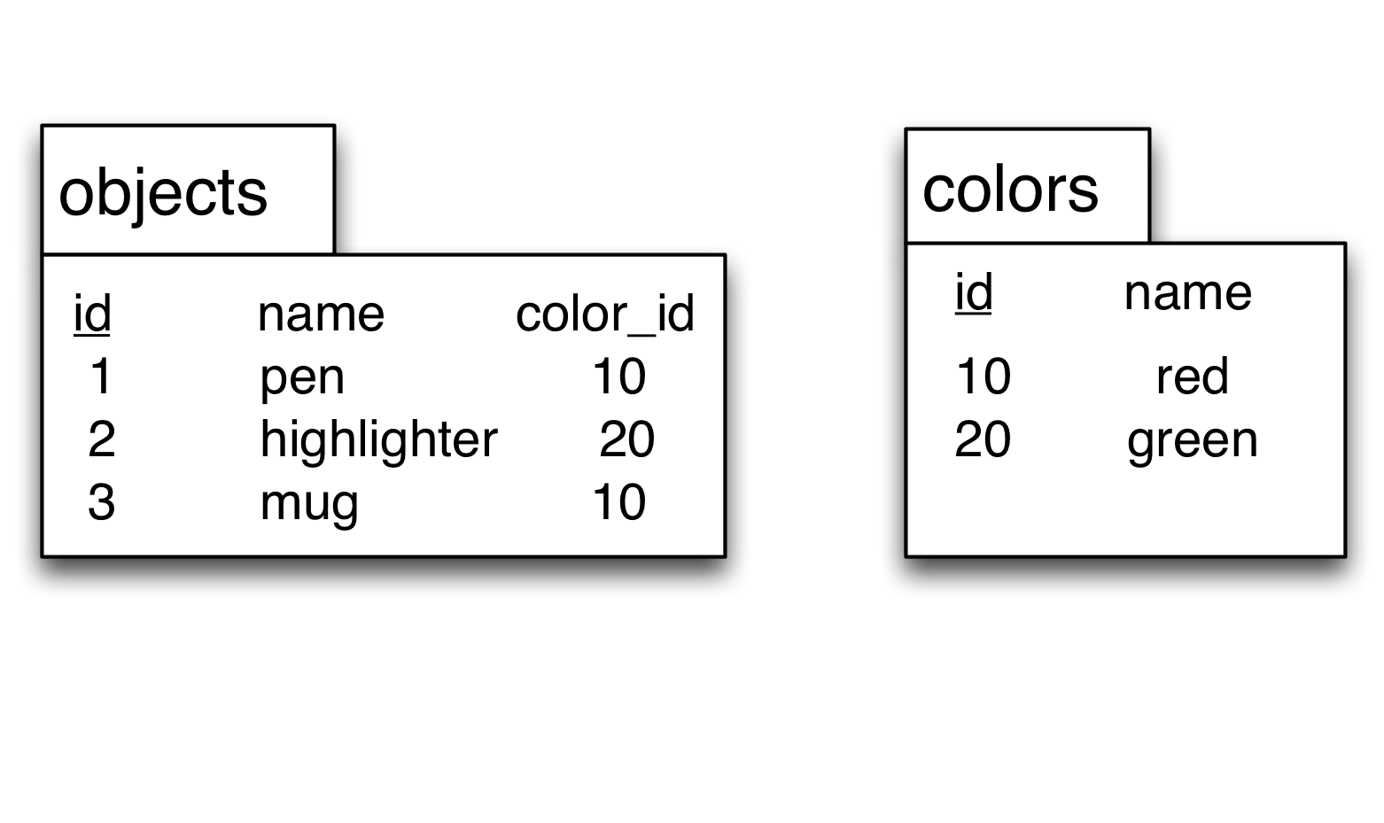
Let’s return to our first database, Objects and Colors:
Now we’re going to add both of these tables into our SQL select statement:
SELECT *
FROM objects, colors
This produces an intermediate table that combines all the rows in objects with all the rows in colors.
Go ahead and try this in datacamp, after uploading colors.csv and objects.csv.
In datacamp you’ll need to specify the files using ‘colors.csv’ etc, and to match the order in the figure use this query:
SELECT *
FROM 'objects.csv', 'colors.csv'
ORDER BY objects.id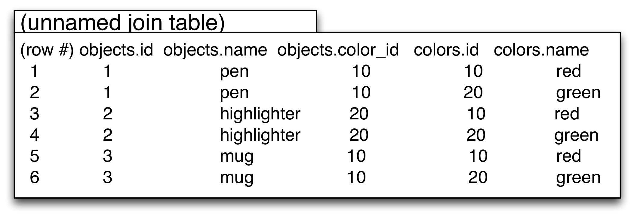
But … that’s odd, because it creates rows that don’t reflect what we know about the objects: the 2nd row talks about a green pen, the 3rd talks about a red highlighter, and the 6th talks about a green mug, none of which actually exist!
On the other hand the table does contain all of the true rows (a red pen, a green highlighter). So what condition might we use to reduce this join table to just the items that make sense in the database?
We need to eliminate the incorrect rows and keep all the true rows. The correct rows all have one thing in common: the value in the objects.color_id column matches the value in the colors.id column. Given that our ids represent the ends of the strings in our original graph database, this makes some sense: the rows we want are the ones that represent the same string (not some weird string that veers off in the middle to connect to another object).
We already know how to eliminate rows based on a condition, using the WHERE clause. Until now, though, we’ve only used WHERE clauses to eliminate rows based on “concrete data” like cars.cyl = 4 or people.name = "Domhog Kwiter". However we can put a column name on either side of the = sign. When we do that we are still asking a single True or False question about each row (not looking at the whole columns), but we’re asking whether the value in one field is the same as the value in the other field (given the values in that row).
So the join condition for linking objects and colors is objects.color_id = colors.id. Working through the rows in the unnamed join table above we use the values in that row:
Row 1: 10 = 10? --> True
Row 2: 10 = 20? --> False
Row 3: 20 = 10? --> False
Row 4: 20 = 20? --> True
...
Visually:
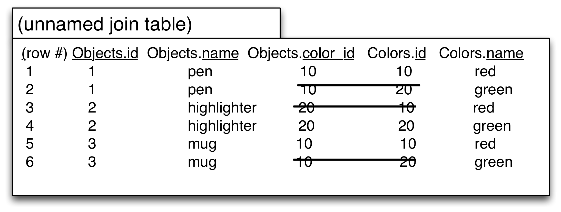
Just as with other conditions in the WHERE clause, only the rows that result in a True are left in the results table.
One way to use the join condition is simply to add it into the WHERE clause, as we would any other condition:
SELECT *
FROM 'objects.csv', 'colors.csv'
WHERE objects.color_id = colors.id
which gives us the results we expect, with only the “correct” rows remaining:
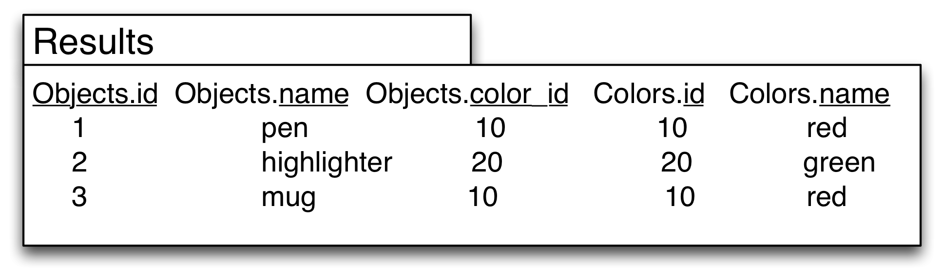
Fantastic, now we know that our pen is red, our highlighter green, and our mug red.
Usually, after we bring together all the data, we want to cut it down further. Remember following the strings from the “red” card to find the names of the red objects? We can do that here, hiding all of the ids. If you look at the join table after the join condition was applied then this is a matter of adding a further condition using AND, just as we would if working with a single table like cars.
SELECT *
FROM 'objects.csv', 'colors.csv'
WHERE objects.color_id = colors.id
  AND colors.name = 'red'
It has been very useful to keep all the columns until this stage, so that we can check that our joins are working correctly (no “incorrect” rows). But we only want the names of the red, so finally we can change the SELECT clause from SELECT * to show just the column we want:
SELECT objects.name
FROM 'objects.csv', 'colors.csv'
WHERE objects.color_id = colors.id
  AND colors.name = 'red'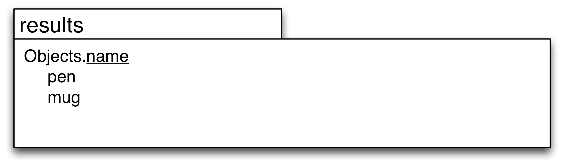
So that’s great, we can now follow the relationships through our database and answer the sorts of questions that people set up databases for in the first place.
The JOIN keyword (old style vs new style joins)
The syntax above works just fine, but it does mix together two different kinds of conditions: we have table joining conditions (objects.color_id = objects.id) and other conditions (objects.color = 'red'). As we’ve seen above these do really work the same, they both eliminate rows from the unnamed (also called cross-product) join table. Nonetheless it can be useful to separate them, which is what the JOIN keyword does, moving the join condition out of the WHERE and into the FROM:
Thus we can re-write:
SELECT *
FROM 'objects.csv', 'colors.csv'
WHERE objects.color_id = colors.id
without a WHERE at all as:
SELECT *
FROM 'objects.csv'
  JOIN 'colors.csv'
    ON objects.color_id = colors.id
And our “only red objects” query could be re-written as:
SELECT objects.name
FROM 'objects.csv'
  JOIN 'colors.csv'
    ON objects.color_id = colors.id
WHERE colors.name = 'red'
In this course we will build our queries like this, noting the number of rows returned each time. If the build up is not step by step I will grade it is incorrect.
SELECT *
FROM 'objects.csv'

-- 3 rows

SELECT *
FROM 'objects.csv'
  JOIN 'colors.csv'
    ON objects.color_id = colors.id

-- shows 3 rows, adding the colors for all objects
SELECT *
FROM 'objects.csv'
  JOIN 'colors.csv'
    ON objects.color_id = colors.id
WHERE colors.name = 'red'

-- Now just 2 rows, removed the green row.

SELECT objects.name
FROM 'objects.csv'
  JOIN 'colors.csv'
    ON objects.color_id = colors.id
WHERE colors.name = 'red'
In this class we will use the JOIN syntax (although it useful to know about the “old-style” syntax, with the join condition in the WHERE).
Sidenote: In the early days of SQL (from the 1970s through mid 1990s) the JOIN keyword did not exist, so join conditions always went into the WHERE clause. That’s why you’ll sometimes hear the JOIN keyword way of doing it called the “new style” and the WHERE way of doing it called the “old style”. Including the join conditions in the WHERE clause is also sometimes called an “implicit join” to emphasize the benefit of JOIN being more explicit. Finally you might hear someone talk about the “comma style” which is the same as the “old-style” not using the JOIN keyword (since the tables are separated by commas).
The JOIN syntax is preferred now because it makes moving to more complicated types of joins easier. OTOH, the comma/old-style syntax always enables one to inspect the intermediate join tables and bridges from the WHERE syntax we learned more clearly. There’s nothing magic about joins, it’s still using conditions on rows.